Download
1 / 31
310 likes | 479 Vues
CORRELATION AND SIMPLE LINEAR REGRESSION - Revisited. Ref: Cohen, Cohen, West, & Aiken (2003), ch. 2. Pearson Correlation. n (x i – m x )(y i – m y )/(n-1) r xy = I=1 _____________________________ = s xy /s x s y s x s y

E N D
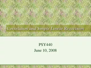
CORRELATION AND SIMPLE LINEAR REGRESSION - Revisited Ref: Cohen, Cohen, West, & Aiken (2003), ch. 2
Pearson Correlation n (xi – mx)(yi – my)/(n-1) rxy = I=1_____________________________ = sxy/sxsy sx sy = zxizyi/(n-1) / = 1 – ( (zxi-zyi)2/2(n-1) = 1 – ( (dzi)2/2(n-1) = COVARIANCE / SDxSDy
Variance of X=1 Variance of X=1 r2= percent overlap in the two squares a. Nonzero correlation B. Zero correlation Variance of Y=1 Variance of Y=1 Fig. 3.6: Geometric representation of r2 as the overlap of two squares
Sums of Squares and Cross Product (Covariance) SSx SSy Sxy
R2 = .42 = .16 .00364 (.40)) .932(.955) SAT Math Calc Grade error Figure 3.4: Path model representation of correlation between SAT Math scores and Calculus Grades
Path Models • path coefficient -standardized coefficient next to arrow, covariance in parentheses • error coefficient- the correlation between the errors, or discrepancies between observed and predicted Calc Grade scores, and the observed Calc Grade scores. • Predicted(Calc Grade) = .00364 SAT-Math + 2.5 • errors are sometimes called disturbances
X Y X Y X Y c a b Figure 3.2: Path model representations of correlation
SUPPRESSED SCATTERPLOT • NO APPARENT RELATIONSHIP Y MALES Prediction lines FEMALES X
IDEALIZED SCATTERPLOT • POSITIVE CURVILINEAR RELATIONSHIP Y Quadratic prediction line Linear prediction line X
Single predictor linear regression. • Regression equations: • y = xb1x+ xb0 • x = yb1y + yb0 • Regression coefficients: • xb1 = rxy sy / sx • yb1 = rxy sx / sy
Two variable linear regression • Path model representation:unstandardized b1 x y e
Linear regression y = b1x + b0 If the correlation coefficient is calculated, then b1 can be calculated from the equation above: b1 = rxy sy / sx The intercept, b0, follows by placing the means for x and y into the equation above and solving: _ _ b0 = y. – [ rxysy/sx ] x.
Linear regression • Path model representation:standardized rxy zy zx e
Least squares estimation The best estimate will be one in which the sum of squared differences between each score and the estimate will be the smallest among all possible linear unbiased estimates (BLUES, or best linear unbiased estimate).
Least squares estimation • errors or disturbances. They represent in this case the part of the y score not predictable from x: • ei = yi – b1xi . • The sum of squares for errors follows: • n • SSe = e2i . • i-1
y e e e e e e e e SSe = e2i x
Matrix representation of least squares estimation. • We can represent the regression model in matrix form: • y = X + e
Matrix representation of least squares estimation • y = X + e • y1 1 x1 e1 • 0 • y2 1 x2 1 e2 • y3 1 x3 e3 • y4 = 1 x4 + e4 • . 1 . . • . 1 . . • . 1 . .
Matrix representation of least squares estimation • y = Xb + e • The least squares criterion is satisfied by the following matrix equation: • b = (X’X)-1X’y . • The term X’ is called the transform of the X matrix. It is the matrix turned on its side. When X’X is multiplied together, the result is a 2 x 2 matrix • n xi • xix2i
SUMS OF SQUARES • SSe = (n – 2 )s2e • SSreg = ( b1 xi – y. )2 • SSy = SSreg + SSe
SUMS OF SQUARES-Venn Diagram ssreg SSy SSx SSe Fig. 8.3: Venn diagram for linear regression with one predictor and one outcome measure
STANDARD ERROR OF ESTIMATE s2y = s2yhat + s2e s2zy = 1 = r2y.x +s2ez sez = sy (1 - r2y.x ) = SSe / (n-2) Review slide 17: this is the standard deviation of the errors shown there
SUMS OF SQUARES- ANOVATable SOURCE df Sum of Mean F Squares Square x 1 SSreg SSreg / 1 SSreg/ 1 SSe /(n-2) e n-2 SSe SSe / (n-2) Total n-1 SSy SSy / (n-1) Table 8.1: Regression table for Sums of Squares
Confidence Intervals Around b and Beta weights sb = (sy / sx ) (1 - r2y.x )/ (n-2) Standard deviation of sampling error of estimate of regression weight b sβ = (1 - r2y.x )/ (n-2) Note: this is formally correct only for a regression equation, not for the Pearson correlation
Distribution around parameter estimates: b-weight ± t sb sb bestimate
Hypothesis testing for the regression weight Null hypothesis: bpopulation = 0 Alternative hypothesis: bpopulation≠ 0 Test statistic: t = bsample / seb Student’s t-distribution with degrees of freedom = n-2
SPSS Regression Analysis option predicting Social Stress from Locus of Control in a sample of 16 year olds Test of b=0 rejected at .05 level
b β R2 = .291 √1- R2 = .842 se .190 (.539)) 3.12(.842) Locus of Control error Social Stress Figure 3.4: Path model representation of prediction of Social Stress from Locus of Control
Difference between Independent b-weights Compare two groups’ regression weights to see if they differ (eg. boys vs. girls) Null hypothesis: bboys = bgirls Test statistic: t = (bboys - bgirls) / (sbboys – bgirls) (sbboys – bgirls) = √ s2bboys+ s2bgirls Student’s t distribution with n1+ n2 - 4
boys n=22 girls n=12 t = ( .281 - .106) / √ (.0812 + .0582 ) = 1.76