Download

1 / 86
1.08k likes | 1.69k Vues
Hartree-Fock Theory. The orbitalar approach. spin. Slater. Mulliken. Combination of Slater determinants. Y (1,….N) = P i f i (i). Pauli principle. Solutions for S 2. MO approach.

E N D
The orbitalar approach spin Slater Mulliken Combination of Slater determinants Y(1,….N) = Pifi(i) Pauli principle Solutions for S2
MO approach We are looking for wavefunctions for a system that contains several particules. We assume that H can be written as a sum of one-particle Hi operator acting on one particle each. H = Si Hi Y(1,….N) = Pifi(i) E = Si Ei A MO is a wavefunction associated with a single electron. The use of the term "orbital" was first used by Mulliken in 1925. Robert Sanderson Mulliken 1996-1986 Nobel 1966
Approximation of independent particles Hartree Fock Fi = Ti + Sk Zik/dik+ Sj Rij Each one electron operator is the sum of one electron terms + bielectronic repulsions 1927 Rij is the average repulsion of the electron j upon i. The self consistency consists in iterating up to convergence to find agreement between the postulated repulsion and that calculated from the electron density. This ignores the real position of j vs. i at any given time.
Self-consistency Given a set of orbitals Y°i, we calculate the electronic distribution of j and its repulsion with i. This allows expressing and solving the equation to find new Y1i allowing to recalculate Rij. The process is iterated up to convergence. Since we get closer to a real solution, the energy decreases. Fi = Ti + Sk Zik/dik+Sj Rij
Assuming Y= Y1Y2 Jij, Coulombic integral for 2 e Let consider 2 electrons, one in orbital Y1, the other in orbital Y2, and calculate the repulsion <1/r12>. Assuming Y= Y1Y2 This may be written Jij = = < Y1Y2IY1Y2> = (Y1Y1IY2Y2) Dirac notation used in physics Notation for Quantum chemists
Assuming Y= Y1Y2 Jij, Coulombic integral for 2 e Jij = < Y1Y2IY1Y2> = (Y1Y1IY2Y2) means the product of two electronic density Coulombic integral. This integral is positive (it is a repulsion). It is large when dij is small. When Y1 are developed on atomic orbitals f1, bilectronic integrals appear involving 4 AOs (pqIrs)
Assuming Y= Y1Y2 Jij, Coulombic integral involved in two electron pairs electron 1: Y1 or Y1 interacting with electron 2: Y2 or Y2 When electrons 1 have different spins (or electrons 2 have different spins) the integral = 0. <aIb>=dij. Only 4 terms are 0 and equal to Jij. The total repulsion between two electron pairs is equal to 4Jij.
Particles are electrons!Pauli Principle electrons are indistinguishable: |Y(1,2,...)|2 does not depend on the ordering of particles 1,2...: | Y (1,2,...)|2 = | Y (2,1,...)|2 Wolfgang Ernst Pauli Austrian 1900 1950 Thus either Y (1,2,...)= Y (2,1,...) S bosons or Y (1,2,...)= -Y (2,1,...) A fermions The Pauli principle states that electrons are fermions.
Particles are fermions!Pauli Principle The antisymmetric function is: YA = Y (1,2,3,...)-Y (2,1,3...)-Y (3,2,1,...)+Y (2,3,1,...)+... which is the determinant Such expression does not allow two electrons to be in the same state the determinant is nil when two lines (or columns) are equal; "No two electrons can have the same set of quantum numbers". One electron per spinorbital; two electrons per orbital. “Exclusion principle”
Two-particle case • The simplest way to approximate the wave function of a many-particle system is to take the product of properly chosen wave functions of the individual particles. For the two-particle case, we have • This expression is a Hartree product. This function is not antisymmetric. An antisymmetric wave function can be mathematically described as follows: • Therefore the Hartree product does not satisfy the Pauli principle. This problem can be overcome by taking a linear combination of both Hartree products • where the coefficient is the normalization factor. This wave function is antisymmetric and no longer distinguishes between fermions. Moreover, it also goes to zero if any two wave functions or two fermions are the same. This is equivalent to satisfying the Pauli exclusion principle.
Generalization: Slater determinant . The expression can be generalized to any number of fermions by writing it as a determinant. John Clarke Slater 1900-1976
Obeying Pauli principleY= 1/√ IY1Y2I Slater determinant Kij, Exchange integral for 2 e Let consider 2 electrons, one in orbital Y1, the other in orbital Y2, and calculate the repulsion <1/r12>. Assuming Y= 1/√ IY1Y2I Kij is a direct consequence of the Pauli principle Kij = = < Y1Y2IY2Y1A> = (Y1Y2IY1Y2) Dirac notation used in physics Notation for Quantum chemists
Obeying Pauli principleY= 1/√ IY1Y2I Slater determinant Kij, Exchange integral It is also a positive integral (-K12 is negative and corresponds to a decrease of repulsion overestimated when exchange is ignored). two electron pairs
Obeying Pauli principleY= 1/√ IY1Y2I Slater determinant Interactions of 2 electrons
Unpaired electrons: sgsu Singlet and triplet statesbielectronic terms │YiYj│+ │YiYj│ Jij+Kij Jij │YiYj│ │YiYj│ Kij Jij-Kij │YiYj│ │YiYj│ │YiYj│- │YiYj│
a(1)a(2) is solution of S2 S2a(1) a(2) = 2a(1) a(2)
a(1)b(2) is not a solution of S2 S2a(1) b(2) = a(1) b(2) + b(1) a(2)
A combination of Slater determinant then may be an eigenfunction of S2 IabI± IbaI = a(1)b(2) a(1)b(2)- b(1)a(2) a(2)b(1) ±b(1)a(2) a(1)b(2)- a(1)b(2) a(2)b(1) + IabI+ IbaI = [a(1)b(2) +b(1)a(2)] (a(1)b(2)- a(2)b(1)) IabI- IbaI = [a(1)b(2) -b(1)a(2)] (a(1)b(2)+ a(2)b(1)) are a eigenfunction of S2 The separation of spatial and spin functions is possible If the spatial function (a or b) is associated with opposite spins
UHF: Variational solutions are not eigenfunctions of S2 Iab’I+ Iba’I = a(1)b’(2) a(1)b(2)- b’ (1)a (2) a(2)b(1) +b(1)a’(2) a(1)b(2)– a’(1)b(2) a(2)b(1) =[a(1)b’(2) +b(1)a’(2)](a(1)b(2)- [a’(1)b(2) +b’(1)a(2)] a(2)b(1)) Not equal The separation of spatial and spin functions is not possible If 2 spatial functions (a a’; b b’) are associated with opposite spins
Electronic correlation • VB method and polyelectronic functions • IC • DFT The charge or spin interaction between 2 electrons is sensitive to the real relative position of the electrons that is not described using an average distribution. A large part of the correlation is then not available at the HF level. One has to use polyelectronic functions (VB method), post Hartree-Fock methods (CI) or estimation of the correlation contribution, DFT.
Electronic correlation A of the correlation refers to HF: it is the “missing energy” for SCF convergence: Ecorr= E – ESCF Ecorr< 0( variational principle) Ecorr~ -(N-1) eV
Importance of correlation effects on Energy Energy (kcal/mol) RHF in blue, Exact in red.
Heitler-London1927 Electrons are indiscernible: If f1(1).f2(2) is a valid solution f1(2).f2(1) also is. The polyelectronic function is therefore: Walter Heinrich Heitler German 1904 –1981 Fritz Wolfgang LondonGerman 1900–1954 [f1(1).f2(2) + f1(2).f2(1)] To satisfy Pauli principle this symmetric expression is associated with an antisymmetric spin function: this represents a singlet state! Each atomic orbital is occupied by one electron: for a bond, this represents a covalent bonding. a (1).b(2) - a(2).b(1)
The resonance, ionic functions Other polyelectronic functions : H1--H2+ H1--H2+ ↔ H1+-H2- f1(1).f1(2) [f1(1).f1(2) + f2(2).f2(1)] symmetric f2(2).f2(1) [f1(1).f1(2) -f2(2).f2(1)] H1+-H2- antisymmetric According to Pauli principle, these functions necessarily correspond to the singlet state: a (1).b(2) - a(2).b(1)
H2 dissociation The cleavage is whether homolytic, H2 → H• + H• or heterolytic: H2 → H+ + H- H+ + H-E = 2 √(1-s)3/p = -0.472 a.u. with s=0.31 H + H E = -1 a.u;
MO behavior of H2 dissociation The cleavage is whether homolytic, H2 → H• + H• or heterolytic: H2 → H+ + H- Energy A-B distance sg2 = (fA +fB)2 = [(fA(1) fA(2) + fB(1) fB(2)] + [(fA(1) fB(2) + fB(1) fA(2)] 50% ionic + 50% covalent The MO description fails to describe correctly the dissociation! su2 = (fA -fB)2 = [(fA(1) fA(2) + fB(1) fB(2)] - [(fA(1) fB(2) + fB(1) fA(2)] 50% ionic - 50% covalent
The Valence-Bond method It consists in describing electronic states of a molecule from AOs by eigenfunctions of S2, Sz and symmetry operators. There behavior for dissociation is then correct. These functions are polyelectronic. To satisfy the Pauli principle, functions are determinants or linear combinations of determinants build from spinorbitals.
Y = IabI + IbaI Y = IabI + IbaI a (1) b(1) IabI = a (2) b(2) Y = IabI - IabI Covalent function for electron pairs Ordered on spins or Ordered on electrons • Y = [a(1).b(2) +a(2). b(1)].[a(1).b(2) - a(2).b(1)] • = [a(1).a(1)b(2)b(2) - b(1).b(1). a(2).a(2)] + [b(1).a(1)a(2)b(2) - a(1).b(1).b(2).a(2)] This is the Heitler-London expression
Interaction Configuration OM/IC: In general the OM are those calculated in an initial HF calculation. Usually they are those for the ground state. MCSCF: The OM are optimized simultaneously with the IC (each one adapted to the state).
Interaction Configuration:mono, di, tri, tetra excitations… Monexcitation: promotion of i to k Diexcitation promotion of i and j to k and l k j i I > ki l k j i k l I j I >
4x4 3x3 2x2 Exact energy levels IC: increasing the space of configuration
Density Functional Theory What is a functional? A function of another function: In mathematics, a functional is traditionally a map from a vector space to the field underlying the vector space, which is usually the real numbers. In other words, it is a function that takes a vector as its argument or input and returns a scalar. Its use goes back to the calculus of variations where one searches for a function which minimizes a certain functional. E = E[r(r)] E(r) = T(r) + VN-e(r) + Ve-e(r)
Thomas-Fermi model (1927): The kinetic energy for an electron gas may be represented as a functional of the density. It is postulated that electrons are uniformely distributed in space. We fill out a sphere of momentum space up to the Fermi value, 4/3 p pFermi3 . Equating #of electrons in coordinate space to that in phase space gives: n(r) = 8p/(3h3) pFermi3 and T(n)=c ∫ n(r)5/3 dr T is a functional of n(r). Llewellen HillethThomas 1903-1992 Enrico Fermi 1901-1954 Italian nobel 1938
DFT Two Hohenberg and Kohn theorems : Pierre C Hohenberg Kohn 1923, german-born american Walter Kohn 1923, Austrian-born American nobel 1998 The existence of a unique functional. The variational principle.
First theorem: on existence The first H-K theorem demonstrates that the ground state properties of a many-electron system are uniquely determined by an electron density. It lays the groundwork for reducing the many-body problem of N electrons with 3N spatial coordinates to only 3 spatial coordinates, through the use of functional of the electron density. This theorem can be extended to the time-dependent domain to develop time-dependent density functional theory (TDDFT), which can be used to describe excited states. The external potential, and hence the total energy, is a unique functional of the electron density.
First theorem on Existence : demonstration The external potential, and hence the total energy, is a unique functional of the electron density. The proof of the first theorem is remarkably simple and proceeds by reductio ad absurdum. Let there be two different external potentials, V1 and V2 , that give rise to the same density r. The associated Hamiltonians,H1 and H2, will therefore have different ground state wavefunctions, Y1 and Y2, that each yield r. E1< < Y2 IH 1I Y2 > = < Y2 IH 2I Y2 > + < Y2 IH1 -H 2I Y2 > = E2 +∫r(r)(V1(r)- V2(r))dr E2< < Y1 IH 2I Y1 > = E1 +∫r(r)(V2(r)- V1(r))dr E1 +E2 <E1 +E2 Therefore ∫r(r)(V1(r)- V2(r))dr=0 and V1(r) = V2(r) The electronic energy of a system is function of a single electronic density only.
Second theorem: Variational principle • The second H-K theorem defines an energy functional for the system and proves that the correct ground state electron density minimizes this energy functional : • If r(r) is the exact density, E[r(r)] is minimum and we search for r by minimizing E[r(r)] with ∫r(r)dr = N • r(r) is a priori unknown • As for HF, the bielectronic terms should depend on two densities ri(r) and rj(r) : the approximation r2e(ri,rj) = ri(ri) rj(rj) assumes no coupling.
Kohn-Sham equations 3 equations in their canonical form: Lu Jeu Sham San Diego Born in Hong-Kong member of the National Academy of Sciences and of the Academia Sinica of the Republic of China
Kohn-Sham equations Equation 1: This reintroduces orbitals: the density is defined from the square of the amplitudes. This is needed to calculate the kinetic energy.
Kohn-Sham equations Equation 2: Using an effective potential, one has a one-body expression. The intractable many-body problem of interacting electrons in a static external potential is reduced to a tractable problem of non-interacting electrons moving in an effective potential. The effective potential includes the external potential and the effects of the Coulomb interactions between the electrons, e.g., the exchange and correlation interactions.
Kohn-Sham equations Equation 3: the writing of an effective single-particle potential Eeff(r) = <Y│Teff+Veff │ Y > Teff+Veff = T + Vmono + RepBi Veff = Vmono + RepBi + T – Teff Veff(r)= V(r)+ ∫e2r(r’)/(r-r’) dr’ + VXC[r(r)] Aslo a mono electronic expression Unknown except for free electron gas as in HF
Exchange correlation functionalsVXC[r(r)] This term is not known except for free electron gas: LDA EXC[r(r)] = ∫r(r) EXC(r) dr EXC[r(r)] = VXC[r(r)]/ r(r) = EXC(r) + r(r) EXC(r)/ r EXC(r) = EX(r) + EC(r) = -3/4(3/p)1/3r(r) + EC(r) determined from Monte-Carlo and approximated by analytic expressions
Exchange correlation functionalsSCF-Xa The introduction of an approximate term for the exchange part of the potential is known as the Xa method. VXa() = -6a(3/4 pr )1/3 r is the local density of spin up electrons and a is a variable parameter. with a similar expression for r↓
Exchange correlation functionalsVXC[r(r)] EXC = EXC(r)LDA or LSDA (spin polarization) EXC = EXC(r,r)GGA or GGSDA - Perdew-Wang - PBE: J. P. Perdew, K. Burke, and M. Ernzerhof EXC = EXC(r,r,Dr)metaGGA
Hybrid methods:B3-LYP (Becke, three-parameters, Lee-Yang-Parr) Incorporating a portion of exact exchange from HF theory with exchange and correlation from other sources : a0=0.20 ax=0.72 aC=0.80 List of hybrid methods: B1B95 B1LYP MPW1PW91 B97 B98 B971 B972 PBE1PBE O3LYP BH&H BH&HLYP BMK Axel D. Becke german 1953
Robert G. Parr Chicago 1921 Chengteh Lee received his Ph.D. from Carolina in 1987 for his work on DFT and is now a senior scientist at the supercomputer company Cray, Inc. Weitao Yang Duke university USA Born 1961 in Chaozhou, China got his undergraduate degree at the University of Peking
DFT Advantages : much less expensive than IC or VB. adapted to solides, metal-metal bonds. Disadvantages: less reliable than IC or VB. One can not compare results using different functionals*. In a strict sense, semi-empical,not ab-initio since an approximate (fitted) term is introduced in the hamiltonian. * The variational priciples applies within a given functional and not to compare them. The only test for validity is comparison with experiment, not a global energy minimum!