Download
1 / 32
400 likes | 855 Vues
Friction: Coulomb’s Law. Static friction force balances pulling force, up to maximum specified by static friction coefficient. Once object begins moving, frictional force drops to constant value, called sliding friction or kinetic friction. Friction Force. Pulling force.

E N D
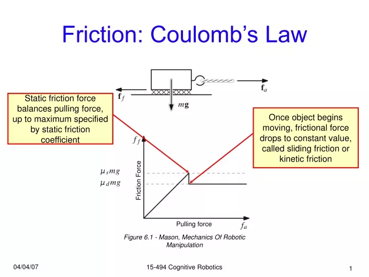
Friction: Coulomb’s Law Static friction force balances pulling force, up to maximum specified by static friction coefficient Once object begins moving, frictional force drops to constant value, called sliding friction or kinetic friction Friction Force Pulling force Figure 6.1 - Mason, Mechanics Of Robotic Manipulation
Friction: Coulomb’s Law For common tasks, independent of velocity and surface area With extreme pressures, coefficient rises With extreme velocities, coefficient drops Coefficients of friction are different for every pair of surfaces — table lookup also differ for every change in temperature, humidity, dust/dirt, vibration, celestial alignment, etc. — not terribly accurate
Friction within Joints Static friction is a headache for fine motor control motor has to ramp up power to overcome static friction within gears, but as soon as it succeeds in doing so, it’s now providing too much power and will “jump” to life. this is the fundamental reason you see the Aibo’s joints twitch from time to time the higher the gear ratio, the bigger the problem
Computing with Forces Forces are defined by a line through space, and a magnitude usually represented by a vector and a point but the point is not unique — any point along the vector is equally valid (“line of action”) Figure 5.1 - Mason, Mechanics Of Robotic Manipulation
Friction with Objects Now we can define a friction cone: Edges of the cone define maximum angle allowed for forces without slippage If you break applied force into normal force fn and tangental force ft, friction cone is defined as |ft| ≤ µ|fn|, with interior angle 2 tan-1µ lL lR fn ft
Friction with Objects Remember Reuleaux’s Method? Works with friction cones as well Now we’re analyzing forces, not displacements, a different interpretation!(be careful about trying to mix them...) Only forces which agree with the all of the contacts’ constraints can be applied by the contact(s): lL lR – + – +
Combining Forces Adding multiple contacts allows you to apply any force in the linear span of their friction cones Remember that forces act along a line through space slide forces along line of action to intersection Resultant force is the vector sum of the two forces, acting through common intersection f2 f1 f1 + f2
Friction with Objects:Examples YES NO NO Don’t actually care about the object itself once contacts have been analyzed – YES + NO YES YES NO YES For reference: – +
Center of Friction Similar to center of mass, center of friction is the integrated pressure over the support region Allows you to treat the interaction as a single contact Hard to model — with a rigid body, small variances completely throw off pressure distribution Ever play Jenga?
Applying Friction & Forces Use weight to flip brick Use wall to direct ball (extra arm) Get ball away from wall Use wall to align/direct brick Stand bone upright Insert objects without jamming or wedging
The Jacobian Matrix One of the most important tools in analyzing and controlling robot motion! Provides the instantaneous velocity in each of the 6 freedoms (translation and orientation along/around each of x, y, and z) as a function of each of the robot’s links = Jacobian (6×n) — a function of current joint positions (q) = joint velocity vector (length n) = workspace velocity vector (length 6)
The Jacobian Matrix:Usage Find current workspace velocity/force Determine contribution ofindividual joints Analyze rank to detect singularities (for better or worse) a singularity occurs when joints become aligned, causing a loss in effector mobility (but increased strength along that axis!) under-actuated robots always haveincomplete rank Full (planar) mobility Singularity:cannot move along y axis, but also don’t have to do any work to resist forces along it
The Jacobian Matrix:Usage Things to watch out for at/near singularities: Small workspace movements/forces may require instantaneous joint motion (infinite motor torque!) Usually occur at workspace limits May have infinite inverse kinematic solutions Test for configuration “quality”: M(q) becomes zero at singularities Swap J(q) and JT(q) if under-actuated (i.e. J(q) is less than full rank)
The Jacobian Matrix:Composition Jacobian is split into two components: = Position component (sometimes ) = Orientation component = Linear velocity vector of end effector = Angular velocity vector of end effector
The Jacobian Matrix:Position Component Remember that a joint’s z axis is always defined to point along its axis of motion If Joint i is prismatic: If Joint i is revolute: Where: zi = z axis of joint i p = position of the end effector pi = position of joint i’s origin (all relative to base frame)
The Jacobian Matrix:Orientation Component If Joint i is prismatic: If Joint i is revolute:
The Jacobian Matrix:Example A planar RRR arm These are all given to you by the forward kinematics: each joint’s transformation matrix holds the current z vector in the 3rd column and the current position in the 4th column
The Jacobian Matrix:Example Notation: s1 = sin(θ1) c123 = cos(θ1+θ2+θ3) A planar RRR arm
The Jacobian Matrix:Example Notation: s1 = sin(θ1) c123 = cos(θ1+θ2+θ3) A planar RRR arm
Dynamics How will joints move as power is applied? Ideally, the robot manufacturer tells you: Inertia Tensor ( , 3×3 matrix) for each link: angular momentum can then be found: Motor properties for each joint: rotor inertia (Im), gear ratio, viscous and coulomb friction Sony isn’t ideal – we don’t have these parameters Aibo doesn’t give direct control over torque anyway (we specify position, it computes power)
Control So then, how does it compute the power for each joint? We want to move the joint to a specified position, and hold it there Sounds easy, right? Harder than it sounds: there may be other forces acting on the joint (e.g. gravity, inertia, etc.) you’re controlling acceleration, two derivatives away from position — go fast, but don’t oscillate
Proportional Control Here’s an idea: take the current position error (e(t) = x(t) - xtgt) multiply e(t) by some parameter kp use this value as the new power outputoutput = -kp· e(t) Should work, right? Farther away means more power. As we get closer, reduce power.
Proportional Control Here’s the resulting graph of position over time: Whoa, look at that oscillation, and it isn’t even oscillating around the right value! One thing at a time buckaroo – oscillation first
PD Control The oscillation is caused because there’s nothing to cause it to slow down as it’s approaching the target — inertia will keep the link moving and blow right past the target if you have significant friction or little inertia (with a speed limit), this may not be a problem Add a braking factor kd, multiplied by the current error derivative ∂e(t)output = -(kp· e(t)) - (kd· ∂e(t))
PD Control Here’s a new graph of position over time: Closer! Now, let’s take care of that offset.
PID Control That offset is caused by external forces, like gravity. We need another term to handle its constant input to our system. Use an integral of the error term, and multiply it by a new coefficient ki:output = -(kp· e(t)) - (ki· ∫e(t)dt) - (kd· ∂e(t)) Actual implementations vary in the parameterization, many use:output = -kp· (e(t) + (ki· ∫e(t)dt) + (kd· ∂e(t)))
PID Control Now look at the graph: Ta-da!
PID Control We’ve put an Excel spreadsheet for this simulation online so you can play with it
Qualifications The graphs shown previously were based on a system with inertia If the system you are controlling does not have inertia, or equivalently, you are controlling velocity directly (not force), proportional control may be all you need! Proportional control often used as a potential field function for steering mobile robots...
Downside of the I Parameter If grasping an object with several manipulators, any error in the manipulator’s position will cause gradually increasing internal strain This is why the Aibo will sometimes shutdown with a joint overload error, simply from standing idly on the ground
The Dirty Little Secret How do we pick the P, I, and D parameters? Hard way: lots of math (a lecture unto itself) Read up on: Laplace Transforms, characteristic equations, pole placement, bode plots Easy way: play with them until you get something you like be careful not to make big changes at a time — don’t want to get into unstable feedback loops Smart way: adaptive self-tuning
Intuitive PID Tuning Advice In our notation (which I believe the AIBO uses) Scaling all the parameters together will scale maximum power output without changing control style (very much) — in the alternative formulation, only P can be scaled this way. P tends to have the biggest impact — higher P means more power , but more oscillation D balances oscillation, but reduces top speed I balances final errors (remember joint twitching?)