Lecture 7: Word Sense Disambiguation (Chapter 7 of Manning and Schutze)

1. Lecture 7: Word Sense Disambiguation(Chapter 7 of Manning and Schutze) Wen-Hsiang Lu (盧文祥) Department of Computer Science and Information Engineering, National Cheng Kung University 2008/11/3 (Slides from Dr. Mary P. Harper, http://min.ecn.purdue.edu/~ee669/) EE669: Natural Language Processing

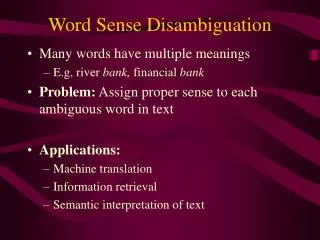
2. Overview of the Problem • Problem:many words have different meanings or senses, i.e., there is ambiguity about how they are to be specifically interpreted (e.g., differentiate). • Task: to determine which of the senses of an ambiguous word is invoked in a particular use of the word by looking at the context of its use. • Note: more often than not the different senses of a word are closely related. EE669: Natural Language Processing

3. Bank The rising ground bordering a lake, river, or sea An establishment for the custody, loan exchange, or issue of money, for the extension of credit, and for facilitating the transmission of funds Title Name/heading of a book, statue, work of art or music, etc. Material at the start of a film The right of legal ownership (of land) The document that is evidence of the right An appellation of respect attached to a person’s name A written work (synecdoche: part stands for the whole) Ambiguity Resolution EE669: Natural Language Processing

4. Overview of our Discussion • Methodology • Supervised Disambiguation: based on a labeled training set. • Dictionary-Based Disambiguation: based on lexical resources such as dictionaries and thesauri. • Unsupervised Disambiguation: based on unlabeled corpora. EE669: Natural Language Processing

5. Methodological Preliminaries • Supervised versus Unsupervised Learning: In supervised learning (classification), the sense label of each word occurrence is provided in the training set; whereas, in unsupervised learning (clustering), it is not provided. • Pseudowords: used to generate artificial evaluation data for comparison and improvements of text-processing algorithms, e.g., replace each of two words (e.g., bell and book) with a pseudoword (e.g., bell-book). • Upper and Lower Bounds on Performance: used to find out how well an algorithm performs relative to the difficulty of the task. • Upper: human performance • Lower: baseline using highest frequency alternative (best of 2 versus 10) EE669: Natural Language Processing

6. Supervised Disambiguation • Training set: exemplars where each occurrence of the ambiguous word w is annotated with a semantic label. This becomes a statistical classification problem; assign w some sense sk in context cl. • Approaches: • Bayesian Classification: the context of occurrence is treated as a bag of words without structure, but it integrates information from many words in a context window. • Information Theory: only looks at the most informative feature in the context, which may be sensitive to text structure. • There are many more approaches (see Chapter 16 or a text on Machine Learning (ML)) that could be applied. EE669: Natural Language Processing

7. Supervised Disambiguation: Bayesian Classification • (Gale et al, 1992): look at the words around an ambiguous word in a large context window. Each content word contributes potentially useful information about which sense of the ambiguous word is likely to be used with it. The classifier does no feature selection; it simply combines the evidence from all features, assuming they are independent. • Bayes decision rule: Decide s’ if P(s’|c) > P(sk|c) for sks’ • Optimal because it minimizes the probability of error; for each individual case it selects the class with the highest conditional probability (and hence lowest error rate). • Error rate for a sequence will also be minimized. EE669: Natural Language Processing

8. Supervised Disambiguation: Bayesian Classification • We do not usually know P(sk|c), but we can use Bayes’ Rule to compute it: • P(sk|c) = (P(c|sk)/P(c)) × P(sk) • P(sk) is the prior probability of sk, i.e., the probability of instance skwithout any contextual information. • When updating the prior with evidence from context (i.e., P(c|sk)/P(c)), we obtain the posterior probability P(sk|c). • If all we want to do is select the correct class, we can ignore P(c). Also use logs to simplify computation. • Assign word w sense s’ = argmaxsk P(sk|c) = argmaxsk P(c|sk) × P(sk) = argmaxsk [log P(c| sk) + log P(sk)] EE669: Natural Language Processing

9. Bayesian Classification: Naïve Bayes • Naïve Bayes: • is widely used in ML due to its ability to efficiently combine evidence from a wide variety of features. • can be applied if the state of the world we base our classification on can be described as a series of attributes. • in this case, we describe the context of w in terms of the words vj that occur in the context. • Naïve Bayes assumption: • The attributes used for classification are conditionally independent: P(c|sk) = P({vj| vj in c}|sk) = vj in cP(vj | sk) • Two consequences: • The structure and linear orderingof words is ignored: bag of words model. • The presence of one word is independent of another, which is clearly untrue in text. EE669: Natural Language Processing

10. Bayesian Classification: Naïve Bayes • Although the Naïve Bayes assumption is incorrect in the context of text processing, it often does quite well, partly because the decisions made can be optimal even in the face of the inaccurate assumption. • Decision rule for Naïve Bayes: Decide s’ if s’ = argmaxsk [log P(sk)+vj in c log P(vj|sk)] • P(vj|sk) and P(sk) are computed via Maximum-Likelihood Estimation, perhaps with appropriate smoothing, from a labeled training corpus. • P(vj|sk) = C(vj,sk)/C(sk) • P(sk) = C(sk)/C(w) EE669: Natural Language Processing

11. Training: for all senses sk of wdo for all vj in vocabulary do P(vj|sk) = C(vj,sk)/C(sk) end end for all senses sk of wdo P(sk) = C(sk)/C(w) end Disambiguation: for all senses sk of wdo score(sk) = log P(sk) for all vj in context window cdo score(sk) = score(sk) + log P(vj|sk) end end chooseargmaxsk score (sk) Bayesian Disambiguation Algorithm Gale, Church, and Yarowsky obtain 90% correct disambiguation on 6 ambiguous nouns in Hansard corpus using this approach (e.g., drug as a medication vs. illicit substance. EE669: Natural Language Processing

12. Supervised Disambiguation:An Information-Theoretic Approach • (Brown et al., 1991) attempt to find a single contextual feature that reliably indicates which sense of an ambiguous word is being used. • For example, the French verbprendre has two different readings that are affected by the word appearing in object position (mesureto take, décisionto make), but the verb vouloir’s reading is affected by tense (present to want, conditional to like). • To make good use of an informant, its values need to be categorized as to which sense they indicate (e.g., mesureto take, décisionto make); Brown et al. use the Flip-Flop algorithm to do this. EE669: Natural Language Processing

13. Supervised Disambiguation:An Information-Theoretic Approach • Let t1,…, tm be translations for an ambiguous word and x1,…, xn be possible values of the indicator. • The Flip-Flop algorithm is used to disambiguate between the different senses of a word using mutual information: • I(X;Y)=xXyY p(x,y) log p(x,y)/(p(x)p(y)) • See Brown et al. for an extension to more than two senses. • The algorithm works by searching for a partition of senses that maximizes the mutual information. The algorithm stops when the increase becomes insignificant. EE669: Natural Language Processing

14. H(X,Y) H(X|Y) I(X; Y) H(Y|X) H(Y) H(X) Mutual Information • I(X; Y)=H(X)-H(X|Y)=H(Y)-H(Y|X), the mutual informationbetween X and Y, is the reduction in uncertainty of one random variable due to knowing about another, or, in other words, the amount of information one random variable contains about another. EE669: Natural Language Processing

15. Mutual Information (cont) • I(X; Y) is symmetric, non-negative measure of the common information of two variables. • Some see it as a measure of dependence between two variables, but better to think of it as a measure of independence. • I(X; Y) is 0 only when X and Y are independent: H(X|Y)=H(X) • For two dependent variables, I grows not only according to the degree of dependence but also according to the entropy of the two variables. • H(X)=H(X)-H(X|X)=I(X; X)  Why entropy is called self-information. EE669: Natural Language Processing

16. The Flip-Flop Disambiguation Algorithm Find random partition P={P1, P2} of translations {t1, …, tm} while (there is a significant improvement) do • find partition Q={Q1, Q2} of indicators {x1, …, xn} that maximizes I(P;Q) • find partition P={P1, P2} of translations {t1, …, tm} that maximizes I(P;Q) end • I(X; Y) = åxXåyYp(x,y) log (p(x,y)/(p(x)p(y))) • Mutual information increases monotonically in the Flip-Flop algorithm, so it is reasonable to stop when there is only an insignificant improvement. EE669: Natural Language Processing

17. Example • Suppose we want to translate prendre based on its object and have {t1, …, tm}={take, make, rise, speak} and {x1, …, xn}={mesure, note, exemple, décision, parole}, and that prendre is used astake when occurring with the objects mesure, note, and exemple; otherwise used as make, rise, or speak. • Suppose the initial partition is P1={take, rise} and P2={make, speak}. • Then choose partition of Q of indicator values that maximizes I(P;Q), say Q1={mesure, note, exemple} and Q2={décision, parole} (selected if the division gives us the most information for distinguishing translations in P1 from translations in P2). • prendre la parole isnot translated as rise to speak when it should be; repartition as P1={take} and P2={rise, make, speak}, and Q as previously. This is always correct for take sense. • To distinguish among the others, we would have to consider more than two senses. EE669: Natural Language Processing

18. Flip-Flop Algorithm • A simple exhaustive search for the best partition of French translations and indicator values would take exponential time. • The Flip-Flop algorithm is a linear time algorithm based on Brieman et al.’s (1984) splitting theorem. • Run the algorithm for all possible indicators and choose the indicator with the highest mutual information • Once the indicator and partition of its values is determined, disambiguation is simple: • For each ambiguous word, determine the value xi of the indicator • If xi is in Q1, assign sense 1; if xi is in Q2, assign sense 2 • Brown et al. (1991) obtained a 20% improvement in MT system using this approach (translations used as senses). EE669: Natural Language Processing

19. Dictionary-Based Disambiguation • If we have no information about the senses of specific instances of words, we can fall back on a general characterization of the senses provided by a lexicon. • We will be looking at three different methods: • Disambiguation based on sense definitions in a dictionary (Lesk, 1986) • Thesaurus-based disambiguation (Walker, 1987 and Yarowsky, 1992) • Disambiguation based on translations in a second-language corpus (Dagan and Itai, 1994) • Also, we will learn about how a careful examination of the distributional properties of senses can lead to significant improvements in disambiguation. • Ambiguous words tend to be used with only one sense in a given discourse with a given collocate. EE669: Natural Language Processing

20. Sense Definition Disambiguation • (Lesk, 1986) uses the simple idea that a word’s dictionary definitions are likely to be good indicators for the senses they define. • For example, the words in definitions associated with the word cone (seed bearing cone versus ice cream containing cone) can be matched to the words in the definitions of all of the words in the context of the word. • Let D1, D2, …., DK be the definitions of the senses s1, s2, …., sKof an ambiguous word w, each represented as a bag of words in the definition. • Let Evj be the dictionary definition(s) for word vjoccurring in context c of w, represented as a bag of words; if sj1, sj2, …, sjLare the senses of vj, then Evj = jt Djt. EE669: Natural Language Processing

21. Sense Definition Disambiguation • Disambiguate the ambiguous word by choosing the sub-definition of the ambiguous word that has the greatest overlap with the words occurring in its context. Overlap can be measured by counting common words or other types of similarity measures. Comment: Given context c for all senses sk of wdo score(sk) = overlap(Dk, vj in c Evj) end Choose s’=argmaxsk score (sk) EE669: Natural Language Processing

22. Sense Definition Disambiguation • By itself, this method is insufficient to achieve highly accurate word sense disambiguation; Lesk obtained accuracies between 50% and 70% on a sample of ambiguous words. • There are possible optimizations that can be applied to improve the algorithm: • Run several iterations of the algorithm on a text, and instead of using a union of all words Evj occurring in the definition for vj, use only the contextually appropriate definitions based on a prior iteration. • Expand each word in context c with synonyms from a thesaurus. EE669: Natural Language Processing

23. Thesaurus-Based Disambiguation • This approach exploits the semantic categorization provided by a thesaurus (e.g., Roget’s) or lexicon with subject categories (e.g., Longman’s) • The basic idea is that semantic categories of the words in a context determine the semantic category of the context as a whole. This category, in turn, determines which word senses are used. • Two approaches: • (Walker, 87) • (Yarowski, 92) EE669: Natural Language Processing

24. Roget’s Thesaurus EE669: Natural Language Processing

25. Thesaurus-Based Disambiguation • (Walker, 87): each word is assigned one or more subject codes in a dictionary corresponding to its different meanings. • If more than one subject code is found, then assume that each code corresponds to a different word sense. • Let t(sk) be the subject code for sense sk of word w in context c. • Then w can be disambiguated by counting the number of words from the context c for which the thesaurus lists t(sk) as a possible subject code. We select the sense that has the subject code with the highest count. • Black(1988) achieved only moderate success on 5 ambiguous words with this approach (~ 50% accuracies). EE669: Natural Language Processing

26. Thesaurus-Based Disambiguation Walker’s Algorithm comment: Given context c for all senses sk of wdo score(sk) = vj in c(t(sk), vj) end choose s’ = argmaxsk score (sk) • Note that (t(sk), vj) = 1 iff t(sk) is one of the subject codes for vj and 0 otherwise. The score is the number of words compatible with the subject code of sk. • One problem with this algorithm is that a general categorization of words into topics may be inappropriate in a particular domain (e.g., mouse as a mammal or electronic device in the context of computer manual). • Another problem is coverage, e.g., names like Navratilova suggests the topic of sports and yet appear in no lexicon. EE669: Natural Language Processing

27. Thesaurus-Based Disambiguation • (Yarowski, 92) adapted topic classification to a corpus as shown on the next slide. • Adds words to a category tl if they occur more often than chance in the contexts of tl in the corpus. • Uses the Bayes classifier for adaptation and disambiguation. • Compute a score for each pair of a context in the corpus ci (100 word window around word w)and a thesaurus category tl. • Making the Naïve Bayes assumption, then compute score(ci,tl). • Use a threshold  to determine which thesaurus categories are salient in a context (larger value requires good evidence to allow a category). • Adjust the semantic categorization in the thesaurus to the corpus. • If vj is covered in thesaurus then adapt its categories to the corpus, • If vj is not covered, then it is added to the appropriate categories. EE669: Natural Language Processing

28. Yarowsky’s Algorithm comment: categorize contexts based on categorization of words for all contexts ci in the corpus do for all thesaurus categories tldo score(ci,tl) = log (P(ci| tl)/P(ci)) × P(tl) end end t(ci) = {tl | score (ci,tl) > } comment: categorize words based on categorization of contexts for all words vj in the vocabulary do Vj = {c | vj in c} end EE669: Natural Language Processing

29. Yarowsky’s Algorithm for all topics tldo Tl = {c | tl t(c)} end for all words vj, all topics tldo P(vj| tl) = |VjTl|/ j |VjTl| end for all topics tldo P(tl) = j |VjTl|/ l j |VjTl| end comment: disambiguation for all senses sk of w occurring in cdo score(sk) = log P(t(sk)) + vj in c log P(vj |t(sk)) end choose s’=argmaxsk score (sk) EE669: Natural Language Processing

30. Yarowsky’s Algorithm • The method achieves a high accuracy when thesaurus categories and senses align well with topics (e.g., bass, star), but when a sense spreads over topics (e.g., interest), the algorithm fails. • Topic independent distinctions between senses are problematic– when interest means advantage, it is not topic specific. In this case, it makes sense that topic-based classification would not work well. EE669: Natural Language Processing

31. Disambiguation Based on Translations in a Second-Language Corpus • (Dagan & Itai, 91, 91) found that words can be disambiguated by looking at how they are translated in other languages. • The first language is the one we wish to disambiguate senses in. • We must have a bilingual dictionary between the first and second language and a corpus for the second (target) language. • Example: the word interest has two translations in German: • Beteiligung (legal share--50% a interest in the company) • Interesse (attention, concern--her interest in Mathematics). • To disambiguate the word interest, we identify the phrase it occurs in and search a German corpus for instances of that phrase. If the phrase occurs with only one of the translations in German, then we assign the corresponding sense whenever the word appears in that phrase. EE669: Natural Language Processing

32. Dagan & Itai’s Algorithm comment: Given context c in which w occurs in relation R(w, v) for all senses sk of wdo score(sk) = |{cS | w’  T(sk), v’  T (v): R(w’, v’) c}| end choose s’=argmaxsk score(sk) • S is the second-language corpus, T(sk) is the set of possible translations of sense sk, and T(v) is the set of possible translations of v. • The score of a sense is the number of times that one of its translations occurs with the translation of v in the second language corpus. EE669: Natural Language Processing

33. Dagan & Itai’s Algorithm • For example, the relation R could be ‘is-object-of’ to disambiguate interest (showed an interestinteresse zeigen (attention or concern) versus acquire an interestBeteiligungerwerben (legal share)). • The algorithm of Dagan and Itai is more complex than shown here; it disambiguates only if the decision can be made reliably. They estimate the probability of an error and make decisions only when the probability of an error is less than 10%. • If a word w in the first language can be translated two ways in the second language within a given phrase (e.g., stand at w), then if there are 10 for the first and 5 for the second sense, then the probability of error is 5/(10+5) = 0.33. EE669: Natural Language Processing

34. One Sense per Discourse, One Sense per Collocation • (Yarowsky, 1995) suggests that there are constraints between different occurrences of an ambiguous word within a corpus that can be exploited for disambiguation: • One sense per discourse: The sense of a target word is highly consistent within any given document. For example, the word differentiate (calculus vs. biology) when used in one way in discourse is likely to continue being used that way. • One sense per collocation: Nearby words provide strong and consistent clues to the sense of a target word, conditional on relative distance, order, and syntactic relationship. The word senses are strongly correlated with certain contextual features like other words in the same phrase. EE669: Natural Language Processing

35. Yarowsky, 1995 • Yarowsky uses an approach that is similar to Brown et al.’s information theoretic method in that it selects the strongest collocational feature for a particular context and disambiguates using this feature alone. • The features are ranked using the ratio: P(sk1|f)/P(sk2|f), the ratio of the number occurrences with sense sk1 with collocation f divided by the number occurrences with sense sk2 with collocation f (with the possibility of smoothing in the case of sparse data). • Selecting the strongest feature removes the need to combine different sources of evidence (given that independence rarely holds, it may be better to avoid the combination). • Achieves accuracies between 90.6% and 96.5%, with a 27% improvement from adding the discourse constraint. EE669: Natural Language Processing

36. Yarowsky’s (1995) Algorithm comment: Initialization for all senses sk of wdo Fk = the set of collocations in sk’s dictionary definition end for all senses sk of wdo Ek =  end • Fk contains the characteristic collocations of sk, which is initialized using the dictionary definition of sk or from another source. • Ek is the set of the contexts of the ambiguous word w that are currently assigned to sk, which is initially empty. EE669: Natural Language Processing

37. Yarowsky’s (1995) Algorithm comment: One sense per collocation while (at least one Ek changed during the last iteration) do for all senses sk of wdo Ek = {ci | fm : fmcifmFk} end for all senses sk of wdo Fk = {fm | nk P(sk| fm)/ P(sn| fm) >} end end comment: One sense per discourse for all documents dmdo determine the majority sense sk of w in dm assign all occurrences of w in dm sense sk end EE669: Natural Language Processing

38. Unsupervised Disambiguation • It may be useful to disambiguate among different word senses in cases where there are no available lexical resources. • in a specialized domain (e.g., linguistics) • could be quite important for information retrieval in a domain • Of course, it is impossible to do sense tagging in a situation where there is no labeled data; however, it is possible to carry out sense discrimination in a completely unsupervised manner. EE669: Natural Language Processing

39. Unsupervised Disambiguation • Without supporting tools such as dictionaries and thesauri and in the absence of labeled text, we can simply cluster the contexts of an ambiguous word into a number of groups and discriminate between these groups without labeling them. • Context-group discrimination (Schutze, 1998): • Clusters uses of an ambiguous word with no additional knowledge. • For an ambiguous word w with senses s1, …, sk, …, sK, estimate the conditional probability of each word vjoccurring in w’s context being used with sense sk, P(vj|sk). EE669: Natural Language Processing

40. Schutze (1998) • The probabilistic model is the same Bayesian model as the one used by Gale et al.’s Bayes classifier, except that each P(vj|sk) is estimated using the EM algorithm. • Start with a random initialization of the parameters of P(vj|sk). • Compute for each context ci of w, the probability P(ci|sk) generated by sk.. • Use this preliminary categorization of contexts as our training data and then re-estimate P(vj|sk) to maximize the likelihood of the data given the model. • EM is guaranteed to increase the log likelihood of the model given the data at each step; therefore, the algorithm stops when the likelihood does not increase significantly. EE669: Natural Language Processing

41. EM Algorithm (Schutze,1998) EE669: Natural Language Processing

42. Schutze (1998) • Once model parameters are estimated, we can disambiguate contexts of w by computing the probability of each of the senses based on the words vj occurring in context. Schutze (1998) uses the Naïve Bayes decision rule: • Decide s’ if s’ = argmaxsk [log P(sk)+vj in c log P(vj|sk)] • The granularity of senses of a word can be chosen by running the algorithm over a range of values. • The larger the number of senses the better it will be able to explain the data. • Relative increase in likelihood may help to distinguish important senses from random variations. • Could make # of senses dependent on the amount of training data. • Can get finer grained distinctions than in supervised approaches. • Works better for topic-dependent senses than topic-independent ones. EE669: Natural Language Processing

43. So What is a Word Sense Really? • It might seem reasonable to define word senses as the mental representations of different word meanings. • Not much is known about mental representations because it is hard to design experiments to get at what that is. • Humans can categorize word usage using introspection, but is that reasonable? Also agreement tends to be low. • Humans could label word senses using dictionary definitions, but this works best for skewed distributions where one sense is predominant. Also, definitions can often be vague. • Words with the highest frequencies have the highest disagreement rate, so selecting words based on frequency would bias results. EE669: Natural Language Processing

44. So What is a Word Sense Really? • It may be that it is common for humans to have a simultaneous activation of different senses when comprehending words in text or discourse (leading to high levels of disagreement). • These coactivations may be cases of systematic polysemy, where lexico-semantic rules apply to the class of words to systematically change or extend their meaning. For example, competition can refer to the act of X or the people doing X. • Proper nouns also create problems, e.g., Brown, Army, etc. • Could consider only coarse-grained distinctions among word senses (like those that show up across languages). Clustering approaches to word sense disambiguation adopt this strategy. EE669: Natural Language Processing

45. Word Sense Disambiguation Evaluation • If the disambiguation task is embedded in a task like translation, then it is easy to evaluate in the context of that application. This leads to application-oriented notions of sense. • Direct evaluation of disambiguation accuracy is more difficult in an application-independent sense. It would be easier if there were standard evaluation sets (Senseval project is addressing this need). • There is a need for researchers to evaluate their algorithms on a representative sample of ambiguous words. EE669: Natural Language Processing

46. Factors Influencing the Notion of Sense • The type of information used in disambiguation affects the notion of sense used: • Co-occurrence (bag-of-words model): topical sense • Relational information (e.g., subject, object) • Other grammatical information (e.g., part-of-speech) • Collocations (one sense per collocation) • Discourse (one sense per discourse segment): How much context is needed to determine sense? • Combinations of the above • Different types of information may be more useful for different parts of speech (e.g., verb meaning is affected by its complements, but nouns are more affected by wider context). EE669: Natural Language Processing