Download

1 / 44
440 likes | 446 Vues
Improved jet clustering algorithm with vertex information for multi-b final states. Taikan Suehara, Tomohiko Tanabe, Satoru Yamashita (The Univ. of Tokyo). TeV physics in ILC/LHC/…. Higgs SUSY exotics. bb (2-jet), WW (up to 4-jet). ex. missing + W (2-jet): 4-jet in pair production.

E N D
Improved jet clustering algorithmwith vertex informationfor multi-b final states Taikan Suehara, Tomohiko Tanabe, Satoru Yamashita(The Univ. of Tokyo)
TeV physics in ILC/LHC/… Higgs SUSY exotics bb (2-jet), WW (up to 4-jet) ex. missing + W (2-jet): 4-jet in pair production Final states with many jets (4/6/8/…) Jet clustering is a major performance driver ILC 2-jet event (ZZ) ILC 6-jet event (ZHH)
Example: ZHH in ILC HHH coupling: a key to prove Higgs mechanism mH=120 GeV Double Higgs-strahlung: largest xsec around 500 GeV Extremely small cross section of 0.2fbBackground (esp. top-pair) must bevery strongly suppressed Excellent b-tag in 6-jet environment
‘# of b jets’ in ZHH Jet clustering(Durham 6-jets) Number of jetscontainingMC b-hadrons # jets including MC b-hadron # of b-jets is reduced due to mis-jet-clustering Major problem in counting b-quarks
New idea: use vertices in jet clustering Jet A(b-jet) ex. bbqq with a hard gluon with 4-jet configuration Jet B (b-jet) c c b b IP Jet C Jet E(gluon jet from D) Jet D
New idea: use vertices in jet clustering Jet A(b-jet) ex. bbqq with a hard gluon with 4-jet configuration Jet B (b-jet) Standard jet clustering: A and B might be combined while E separated c c b b IP Jet C Jet E(gluon jet from D) Jet D
New idea: use vertices in jet clustering Jet A(b-jet) ex. bbqq with a hard gluon with 4-jet configuration Jet B (b-jet) Standard jet clustering: A and B might be combined while E separated c c b Vertex clustering: Two b-jets can be separated with vertex information b IP Jet C Jet E(gluon jet from D) Jet D
New idea: use vertices in jet clustering Jet A(b-jet) ex. bbqq with a hard gluon with 4-jet configuration Jet B (b-jet) Standard jet clustering: A and B might be combined while E separated c c b Vertex clustering: Two b-jets can be separated with vertex information b IP Jet C Jet E(gluon jet from D) Jet D
Sample in MC (2D extraction) Red circle: MC b (before gluon emission), Star: vertex found Triangle: Durham jets, Square: Our jet clustering
Details (a bit) of our method Vertex finder Secondary Muon ID Vertex combination Jet clustering using vertices Jet flavor tagging
1. A new build-up vertex finder High-purity vertex finder is critical in this method Fake vertices significantly degrade performance! Problem: Usual vertex finders assume jet clustering is correct … and use the jet direction to improve purity We cannot use jet direction since we search for vertices first Original vertex finder • Build-up method (pairing tracks -> association) • Not include new idea; main effort on optimization • - mass based cuts, track combination order, etc. For implementation details, see backup slides
2. Secondary muon ID Secondary muons can also be usedto identify heavy-flavor jets • Secondary electrons are currently not used(because of non-trivial separation from pions) Secondary muon criteria: • Require hit in muon detector • Impact parameter > 5 s, < 5 mm • ECAL, HCAL energy deposit Secondary muons are treated similarly tovertices (with muon direction as vtx. direction)
3. Vertex combination Our jet clustering strategy: • Simple combination criteria • Opening angle to IP < 0.2 rad. • In muon case; < 0.3 rad. • Identify heavy flavor jets using vertices • Separate heavy flavor jets using vertices b & c vertices must be combined others must remain separated Wrong combination True combination Secondary vertex IP q Muon direction
4. Jet clustering using vertices • Combined vertices are listed as ‘jet core’ • All particles within 0.2 rad. to the jet core are associated to the core • All associated jet cores and residual particles are associated with Durham y criteria * Jet cores with vertices are never combined to each other (y value is set to +inf.) IP Jet core
4. Jet clustering using vertices • Combined vertices are listed as ‘jet core’ • All particles within 0.2 rad. to the jet core are associated to the core • All associated jet cores and residual particles are associated with Durham y criteria 0.2 rad * Jet cores with vertices are never combined to each other (y value is set to +inf.) assoc. by angle IP
4. Jet clustering using vertices • Combined vertices are listed as ‘jet core’ • All particles within 0.2 rad. to the jet core are associated to the core • All associated jet cores and residual particles are associated with Durham y criteria Durham Nevercombined * Jet cores with vertices are never combined to each other (y value is set to +inf.) IP assoc. by Durham
5. Jet flavor tagging (LCFIVertex) Neural-net based flavor tagging package of standard ILC analysis (now improving also by us, but new version not available yet) b-likeness c-likeness parton charge neural net joint prob. input variables (tracks) input variables (vertex) LCFI Collaboration: NIM A 610 (573) [arxiv:0908.3019]
Performance MC number of b-jets MC number of tracks from b-hadrons ZHH vs. top-pair b-tagging performance Effect on b-tag cut in ZHH analysis
1. MC number of b-jets Quick view of the vertex effect Procedure: • Jet clustering (Durham / Vertex) • Listing b-hadrons (MC information) Listing tracks from b-hadrons • Associate b-hadrons to reconstructed jets Jet including largest # of tracks from a b-hadron is associated to the b-hadron • Counting jets associated to b-hadrons Using ZHH -> bbbbbb events (# b-jets should be 6)
1. MC number of b-jets Durham Vertex # jets including MC b-hadron All jets including b – 52% -> 66% Significant improvement!
2. MC number of tracks from b-hadrons Effect on b-tagging at MC level UsingZHH -> qqHH (H->bb: 68%, Z decays to every flavor) tt -> bbcssc (each W decays to c and s quarks) Procedure: • Listing b-hadron tracks with MC information • Counting b-hadron tracks in each jet • Sort jets by number of b-hadron tracks • See 3rd and 4th jets: • qqHH: #b=4; # b-hadron tracks should be > 0 • tt: #b=2; # b-hadron tracks should be 0
2. MC number of tracks from b-hadrons qqhh (should be non-zero) 4th jet Durham Vertex 3rd jet tt (should be zero) 4th jet 3rd jet qqHH acceptance improved tt rejection improved
3. ZHH vs. top-pair b-tagging performance Study with realistic b-tagging Procedure: • Jet clustering (Durham / Vertex) • Flavor tagging by LCFIVertex • obtain b-likeness value (0 to 1) for each jet • Check qqHH vs bbcssc acceptance with varying b-likeness threshold • Both 3rd and 4th jets and sum b-likeness over all jets are examined Using ZHH -> qqHH & tt -> bbcssc (same as 2.)
3. ZHH vs. top-pair b-tagging performance Durham JC Vertex JC worse better Cut on 4th jet Cut on 3rd jet Cut on sum b-likeness • Improvements seen in all criteria • Improvements are particularly significant for high-purity region (signal eff. < 60%)
4. Effect on b-tag cut in ZHH analysis Practical impact on the physics study • Jet clustering & flavor tagging • Determine cut value of b-likenessat signal efficiency = 50% • High purity is neededto suppress enormous tt background • Count the remaining number of eventsand scale to 1 ab-1 luminosity Using ZHH -> qqHH & tt -> bbcssc (same as 2. & 3.)
4. Effect on b-tag cut in ZHH analysis Numbers in parentheses are at 1 ab-1 Vertex jet clustering Durham jet clustering 30% improvement!
Summary Vertex clustering can improve jet clustering performance for counting b-jets Simple analysis with ZHH shows 30% improvement in reducing tt background
Backup • ILD detector • ZHH analysis by J. Tian • Vertex finder details • LCFIVertex input variables
ILD Detector muon detector hadron calorimeter em calorimeter TPC vertex detector beam pipe TPC + VXD are critical for flavor tagging!
J.Tian, ALCPG 11 s = 0.2 fb: Only 100 events in 500 fb-1
qqhh (without Z-like pair) ttbar with mis-b-tag
1. Vertex finding (1) • Original jet finder based on “build-up” method • ZVTOP cannot be used without tuning • It’s designed to be used after jet clustering • Too many fakes – without “jet-direction” parameter • IP tracks are firstly removed (tear-down) • Vertices are calculated for every track-pair • Calculate nearest points of two helices • Geometric calculation for the start point • Minuit minimization using track error-matrices
1. Vertex finding (2) • Pre-selection • Mass < 10 GeV (B: ~5 GeV) • Momentum & vertex pos: not opposite to IP • Vertex mass < energy of either track • This selection is very effective for dropping fakes • Vertex distance to IP > 0.3 mm • Track chi2 to the vertex < 25 • Associate more tracks to passed vertices • Using same criteria as above • Sort & select obtained vertices by probability • Associated (# tracks >=3) vertices are prioritized • Example in next slide…
1. Vertex finding (3) • Example: 5 vertices are found
1. Vertex finding (3) • Example Adopted! Removed!
1. Vertex finding (3) • Example Adopted!
1. Vertex finding (3) • Example Adopted! Adopted! Removed!
1. Vertex finding (3) • Example Finally, three vertices are adopted. Adopted! Adopted! Adopted!
Vertices in ZHH -> bbbbbb Wrong vertices True vertices Vertex position [mm] In 347 bbbbbb events: Good = 2040, bad (not from B-semistable) = 90
2. Vertex selection & muons • Vertex selection • K0 vertices are removed (mass +- 10 GeV) • Vertex position > 30 mm are removed • Mostly s-vertices • Secondary muons • Following tracks are treated as same as vertices • With muon hit • Currently > 50 MeV energy deposit • Impact parameter (> 5 sigma & not too much) • Ecal, Hcal energy deposit
Selection performance • Vertex selection (347 bbbbbb events) • Lepton selection (347 bbbbbb events) Optimized for efficiency (bad contains partially bad) Optimized for purity (not so good efficiency)
LCFI input variables • LCFI input variables: • three categories, trained independently: • # vertex = 0 • # vertex = 1 • # vertex >= 2 • for # vertex = 0 (8 variables): • d0 impact parameter (1) • d0 impact parameter (2) • z0 impact parameter (1) • z0 impact parameter (2) • track momentum (1) • track momentum (2) • d0 joint probability • z0 joint probability • for # vertex = 1, >=2 (8 variables): • d0 joint probability • z0 joint probability • vertex decay length • vertex decay length significance • vertex momentum • pt-corrected vertex mass • vertex multiplicity • vertex probability from the fitter (1) and (2) indicate the most and second most significant track. • “joint probability” – probability that a track comes from the IP, computed a priori using the distribution of impact parameter significance (separately for d0 and z0), multiplied for all tracks in the jet