Download
1 / 63
640 likes | 936 Vues
Decidability. The diagonalization method The halting problem is undecidable. Undecidability. decidable. decidable RE all languages our goal: prove these containments proper. all languages. regular languages. context free languages. RE. Countable and Uncountable Sets.

E N D
Decidability The diagonalization method The halting problem is undecidable
Undecidability decidable decidable RE all languages our goal: prove these containments proper all languages regular languages context free languages RE
Countable and Uncountable Sets • the natural numbers N = {1,2,3,…} are countable • Definition: a set S is countable if it is finite, or it is infinite and there is a bijection f: N → S
Example Countable Set • The positive rational numbers Q = {m/n | m, n N } are countable. • Proof: … 1/1 1/2 1/3 1/4 1/5 1/6 … 2/1 2/2 2/3 2/4 2/5 2/6 … 3/1 3/2 3/3 3/4 3/5 3/6 … 4/1 4/2 4/3 4/4 4/5 4/6 … 5/1 …
Example Uncountable Set Theorem: the real numbers R are NOT countable (they are “uncountable”). • How do you prove such a statement? • assume countable (so there exists bijection f) • derive contradiction (some element not mapped to by f) • technique is called diagonalization (Cantor)
Example Uncountable Set • Proof: • suppose R is countable • list R according to the bijection f: n f(n) _ 1 3.14159… 2 5.55555… 3 0.12345… 4 0.50000… …
Example Uncountable Set • Proof: • suppose R is countable • list R according to the bijection f: n f(n) _ 1 3.14159… 2 5.55555… 3 0.12345… 4 0.50000… … set x = 0.a1a2a3a4… where digit ai ≠ ith digit after decimal point of f(i) (not 0, 9) e.g. x = 0.2312… x cannot be in the list!
Non-RE Languages Theorem: there exist languages that are not Recursively Enumerable. Proof outline: • the set of all TMs is countable • the set of all languages is uncountable • the function L: {TMs} →{languages} cannot be onto
Non-RE Languages • Lemma: the set of all TMs is countable. • Proof: • the set of all strings * is countable, for a finite alphabet . With only finitely many strings of each length, we may form a list of * by writing down all strings of length 0, all strings of length 1, all strings of length 2, etc. • each TM M can be described by a finite-length string s <M> • Generate a list of strings and remove any strings that do not represent a TM to get a list of TMs
Non-RE Languages • Lemma: the set of all languages is uncountable • Suppose we could enumerate all languages over {0,1} and talk about “the i-th language.” • Consider the language L = { w | w is the i-th binary string and w is not in the i-th language}.
Lj x j-th Proof – Continued • Clearly, L is a language over {0,1}. • Thus, it is the j-th language for some particular j. • Let x be the j-thstring. • Is x in L? • If so, x is not in L by definition of L. • If not, then x is in L by definition of L. Recall: L = { w | w is the i-th binary string and w is not in the i-th language}.
Proof – Concluded • We have a contradiction: x is neither in L nor not in L, so our sole assumption (that there was an enumeration of the languages) is wrong. • Comment: This is really bad; there are more languages than TM. • E.g., there are languages that are not recognized by any Turing machine.
Non-RE Languages • Lemma: the set of all languages is uncountable • Proof: • fix an enumeration of all strings s1, s2, s3, … (for example, lexicographic order) • a language L is described by its characteristic vector L whose ith element is 0 if si is not in L and 1 if si is in L
Non-RE Languages • suppose the set of all languages is countable • list characteristic vectors of all languages according to the bijection f: n f(n) _ 1 0101010… 2 1010011… 3 1110001… 4 0100011… …
Non-RE Languages • suppose the set of all languages is countable • list characteristic vectors of all languages according to the bijection f: set x = 1101… where ith digit ≠ ith digit of f(i) x cannot be in the list! therefore, the language with characteristic vector x is not in the list n f(n) _ 1 0101010… 2 1010011… 3 1110001… 4 0100011… …
So far… some language decidable • We will show a natural undecidable L next. {anbn | n ≥ 0} all languages regular languages context free languages RE {anbncn | n ≥ 0}
The Halting Problem • Definition of the “Halting Problem”: HALT = { <M, x> | TM M halts on input x } • Is HALT decidable?
The Halting Problem Theorem: HALT is not decidable (undecidable). Proof: • Suppose TM H decides HALT • if M accept x, H accept • if M does not accept x, H reject • Define new TM H’: on input <M> • if H accepts <M, <M>>, then loop • if H rejects <M, <M>>, then halt • consider H’ on input <H’>: • if it halts, then H rejects <H’, <H’>>, which implies it cannot halt • if it loops, then H accepts <H’, <H’>>, which implies it must halt • contradiction. Thus neither H nor H’ can exist
So far… • Can we exhibit a natural language that is non-RE? {anbn | n ≥ 0 } some language decidable all languages regular languages context free languages RE HALT {anbncn | n ≥ 0 }
RE and co-RE • The complement of a RE language is called a co-RE language some language {anbn : n ≥ 0 } co-RE decidable all languages regular languages context free languages RE {anbncn : n ≥ 0 } HALT
RE and co-RE Theorem: a language L is decidable if and only if L is RE and L is co-RE. Proof: () we already know decidable implies RE • if L is decidable, then complement of L is decidable by flipping accept/reject. • so L is in co-RE.
RE and co-RE Theorem: a language L is decidable if and only if L is RE and L is co-RE. Proof: () we have TM M that recognizes L, and TM M’ recognizes complement of L. • on input x, simulate M, M’ in parallel • if M accepts, accept; if M’ accepts, reject.
A natural non-RE Language Theorem: the complement of HALT is not recursively enumerable. Proof: • we know that HALT is RE • suppose complement of HALT is RE • then HALT is co-RE • implies HALT is decidable. Contradiction.
Summary co-HALT some problems have no algorithms, HALT in particular. some language {anbn : n ≥ 0 } co-RE decidable all languages regular languages context free languages RE {anbncn : n ≥ 0 } HALT
Complexity Complexity P、NP、NPC
Complexity • So far we have classified problems by whether they have an algorithm at all. • In real world, we have limited resources with which to run an algorithm: • one resource: time • another: storage space • need to further classify decidable problems according to resources they require
Worst-Case Analysis • Always measure resource (e.g. running time) in the following way: • as a function of the input length • value of the function is the maximum quantity of resource used over all inputs of given length • called “worst-case analysis” • “input length” is the length of input string
Time Complexity Definition: the running time (“time complexity”) of a TM M is a function f: N → N where f(n) is the maximum number of steps M uses on any input of length n. • “M runs in time f(n),” “M is a f(n) time TM”
Analyze Algorithms • Example: TM M deciding L = {0k1k : k ≥ 0}. • On input x: • scan tape left-to-right, reject if 0 to right of 1 • repeat while 0’s, 1’s on tape: • scan, crossing off one 0, one 1 • if only 0’s or only 1’s remain, reject; if neither 0’s nor 1’s remain, accept # steps? # steps? # steps?
Analyze Algorithms • We do not care about fine distinctions • e.g. how many additional steps M takes to check that it is at the left of tape • We care about the behavior on large inputs • general-purpose algorithm should be “scalable” • overhead for e.g. initialization shouldn’t matter in big picture
Measure Time Complexity • Measure time complexity using asymptotic notation (“big-oh notation”) • disregard lower-order terms in running time • disregard coefficient on highest order term • example: f(n) = 6n3 + 2n2 + 100n + 102781 • “f(n) is order n3” • write f(n) = O(n3)
Asymptotic Notation Definition: given functions f, g: N → R+, we say f(n) = O(g(n)) if there exist positive integers c, n0 such that for all n ≥ n0 f(n) ≤ cg(n) • meaning: f(n) is (asymptotically) less than or equal to g(n) • E.g. f(n) = 5n4+27n, g(n)=n4, take n0=1 and c = 32 (n0=3 and c = 6 works also)
Analyze Algorithms • On input x: • scan tape left-to-right, reject if 0 to right of 1 • repeat while 0’s, 1’s on tape: • scan, crossing off one 0, one 1 • if only 0’s or only 1’s remain, reject; if neither 0’s nor 1’s remain, accept • total = O(n) + (n/2)O(n) + O(n) = O(n2) O(n) steps ≤ n/2 repeats O(n) steps O(n) steps
Asymptotic Notation Facts • “logarithmic”: O(log n) • logbn = (log2 n)/(log2 b) • so logbn = O(log2 n) for any constant b; therefore suppress base when write it • “polynomial”:O(nc) = nO(1) • also: cO(log n) = O(nc’) = nO(1) • “exponential”: O(2nδ) for δ > 0
Time Complexity Class • Recall: • a language is a set of strings • a complexity class is a set of languages • complexity classes we’ve seen: • Regular Languages, Context-Free Languages, Decidable Languages, RE Languages, co-RE languages Definition: Time complexity class TIME(t(n)) = {L | there exists a TM M that decides L in time O(t(n))}
Time Complexity Class • We saw that L = {0k1k : k ≥ 0} is in TIME(n2). • It is also in TIME(n log n) by giving a more clever algorithm • Can prove: O(n log n) time required on a single tape TM. • How about on a multitape TM?
Multitaple TMs • 2-tape TM M deciding L = {0k1k : k ≥ 0}. • On input x: • scan tape left-to-right, reject if 0 to right of 1 • scan 0’s on tape 1, copying them to tape 2 • scan 1’s on tape 1, crossing off 0’s on tape 2 • if all 0’s crossed off before done with 1’s reject • if 0’s remain after done with ones, reject; otherwise accept. O(n) O(n) O(n) total: 3*O(n) = O(n)
Multitape TMs • Convenient to “program” multitape TMs rather than single-tape ones • equivalent when talking about decidability • not equivalent when talking about time complexity Theorem: Let t(n) satisfy t(n)≥n. Every t(n) multitape TM has an equivalent O(t(n)2) single-tape TM.
“Polynomial Time Class” P • interested in a coarse classification of problems. • treat any polynomial running time as “efficient” or “tractable” • treat any exponential running time as “inefficient” or “intractable” Definition: “P” or “polynomial-time” is the class of languages that are decidable in polynomial time on a deterministic single-tape Turing Machine. P = k ≥ 1 TIME(nk)
Why P? • insensitive to particular deterministic model of computation chosen (“Any reasonable deterministic computational models are polynomially equivalent.”) • empirically: qualitative breakthrough to achieve polynomial running time is followed by quantitative improvements from impractical (e.g. n100) to practical (e.g. n3 or n2)
Examples of Languages in P • PATH = {<G, s, t> | G is a directed graph that has a directed path from s to t} • RELPRIME = {<x, y> | x and y are relatively prime} • ACFG = {<G, w> | G is a CFG that generates string w}
Nondeterministic TMs • Recall: nondeterministic TM • informally, TM with several possible next configurations at each step
Nondeterministic TMs visualize computation of a NTM M as a tree Cstart • nodes are configurations • leaves are accept/reject configurations • M accepts if and only if there exists an accept leaf • M is a decider, so no paths go on forever • running time is max. path length rej acc
“Nondeterministic Polynomial Time Class” NP Definition: TIME(t(n)) = {L | there exists a TM M that decides L in time O(t(n))} P = k ≥ 1 TIME(nk) Definition: NTIME(t(n)) = {L | there exists a NTM M that decides L in time O(t(n))} NP = k ≥ 1 NTIME(nk)
Poly-Time Verifiers “certificate” or “proof” • NP = {L | L is decided by some poly-time NTM} • Very useful alternate definition of NP: Theorem: language L is in NP if and only if it is expressible as: L = { x | y, |y| ≤ |x|k, <x, y> R } where R is a language in P. • poly-time TM MR deciding R is a “verifier” efficiently verifiable
Example • HAMPATH = {<G, s, t> | G is a directed graph with a Hamiltonian path from s to t} is expressible as HAMPATH = {<G, s, t> | p for which <<G, s, t>, p> R}, R = {<<G, s, t>, p> | p is a Ham. path in G from s to t} • p is a certificate to verify that <G, s, t> is in HAMPATH • R is decidable in poly-time
Poly-Time Verifiers L NP iff. L = { x | y, |y| ≤ |x|k, <x, y> R } Proof: () give poly-time NTM deciding L phase 1: “guess” y with |x|k nondeterministic steps phase 2: decide if <x, y> R
Poly-Time Verifiers Proof: () given L NP, describe L as: L = { x | y, |y| ≤ |x|k, <x, y> R } • L is decided by NTM M running in time nk • define the language R = {<x, y> | y is an accepting computation history of M on input x} • check: accepting history has length ≤ |x|k • check: M accepts x iffy, |y| ≤ |x|k, <x, y> R
Why NP? • not a realistic model of computation • but, captures important computational feature of many problems: exhaustive search works • contains huge number of natural, practical problems • many problems have form: L = { x | y s.t. <x, y> R } object we are seeking efficient test: does y meet requirements? problem requirements
Examples of Languages in NP • A clique in an undirected graph is a subgraph, wherein every two nodes are connected. • CLIQUE = {<G,k> | graph G has a k-clique}