Download
1 / 1
10 likes | 151 Vues
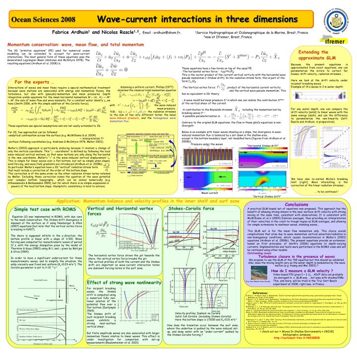
Wave-current interactions in three dimensions. Ocean Sciences 2008. Fabrice Ardhuin 1 and Nicolas Rascle 1,2 , Email : ardhuin@shom.fr, 1 Service Hydrographique et Océanographique de la Marine, Brest, France 2 now at Ifremer, Brest, France.

E N D
Wave-current interactions in three dimensions Ocean Sciences 2008 Fabrice Ardhuin1 and Nicolas Rascle1,2, Email : ardhuin@shom.fr, 1Service Hydrographique et Océanographique de la Marine, Brest, France 2now at Ifremer, Brest, France Momentum conservation: wave, mean flow, and total momentum The 3D “primitive equations” (PE) used for numerical ocean modelling can be extended to account for wave-current interactions. The most general form of these equations uses the Generalized Lagrangian Mean (Andrews and McIntyre 1978). The resulting equations (Ardhuin et al. 2008) is Extending the approximate GLM Because the present equations is approximated from exact equations, one can parameterize the errors to correct for biases: drift velocity, radiation stresses … Here we look at the drift velocity under incipient breaking waves. Example of 14 s waves in 3 m water depth: For any water depth, one can compare the drift velocity (solid) to linear waves with the same energy (dash), and use the difference to parameterize the non-linearity (left: Rascle and Ardhuin, in preparation). We have also re-visited Miche’s breaking limit (right). More interesting, is the correction of the linear radiation stresses… … to be continued ! • These equations have a few terms on top of the usual PE: • The horizontal vortex force : • This is the vector product of the current vertical vorticity with the horizontal wave pseudo-momentum (~Stokes drift). In the radiation stress form, this is part of the term • The Vertical vortex force: , product of the horizontal current vorticity and the vertical wave pseudo-momentum. This has no equivalent in 2D theory. • A wave-modified mean pressure SJ in which one can isolate the contribution Sshear of the vertical shear of the current. • A contribution to the Reynolds stresses including the momentum lost by breaking waves T wc. • A possible parameterization is • Contrary to the original GLM equations, the flow in these glm2z equations is non-divergent. • Below is an example with linear waves shoaling on a slope, the divergence in wave-induced momentum flux is balanced by a set-down in the shallow area… • except in the bottom boundary layer, not modelled here (figures from Ardhuin et al. 2008b). For the experts … Assuming a uniform current, Phillips (1977) obtained the classical total momentum equation • Interactions of waves and mean flows require a special mathematical treatment because wave motions are associated with energy and momentum fluxes, like turbulence, but also with (pseudo)-momentum and mean pressures. Depth integration yields equations for the mean horizontal momentum M = (Mx ,My) = Mm + Mw,the sum of mean flow and wave momenta. For a constant water density w we have (Smith 2006, with the simple addition of the Coriolis force), • These equations use special assumptions and are not easily extended to 3D. • For 3D, two approaches can be followed: • analytical continuation across the surface (e.g. McWilliams & al. 2004) • -> interpretation ?? • surface-following coordinates (e.g. Andrews & McIntyre 1978, Mellor 2003). • Mellor’s (2003) approach is particularly seducing because it involves a change of only the vertical coordinate. This “ - coordinate” is defined by following the local wave-induced vertical motions, so that wave motions are only along the horizontal in the new coordinate. Mellor’s “s” is the wave-induced vertical displacement 3. This is simple for linear waves over a flat bottom, but not so simple when slopes, wind forcing, and wave field gradients are introduced (Ardhuin et al. 2008b). • In particular Mellor’s equation have a 3D “vertical” radiation stress term , • that must include a correction of the order of the bottom slope. • This correction is of the same order as the other radiation stress terms retained by Mellor. Including these correction raises the question of the wave potential over complex bottom topography… which can be solved numerically (e.g. Athanassoulis & Belibassakis 1999), but for which there is no simple expansions in • powers of the local bottom slope. Asymptotic consistency is hard to achieve. with the wave-induced mean pressure N.B.: Srad = SJ+ CgEk/ the radiation stresses re the sum of two very different terms: the mean wave-induced pressure, and the homogenous wave momentum flux. Pressure under the waves “Horizontal Stokes drift” Mean current “Vertical Stokes drift” Application: Momentum balance and velocity profiles in the inner shelf and surf zone Conclusions A practical GLM-based set of equations was proposed. This approach has the benefit of allowing strong shears in the near-surface drift velocity with strong mixing at the same time, consistent with observations. It is consistent with McWilliams et al.’s (2004) Eulerian averages, thus providing an interpretation of their velocities in the crest-to-trough region as GLM averages, and allowing for simple extensions to nonlinear waves, standing waves... This GLM set is for the mean flow momentum only. This choice avoids complications that arise due to wave momentum vertical advection/radiation in non-homogenous conditions, which causes inconsistencies in Mellor’s (2003) equations (Ardhuin et al. 2008b). The present equations provide an extension, based on first principles, of Smith’s (2006) equations to depth-varying currents. Implementation and tests were performed in the ROMS code and will be continued using other models. Outstanding issues Turbulence closure in the presence of waves We propose to use the GLM of the TKE equation but this should be validated. Also, does the mixing length vary as the water depth is modulated by the wave motion (e.g. Huang and Mei 2003) ? How do I measure a GLM velocity ? Video-based PIV gives û + ½ Us… ADCP data can probably be averaged in a GLM way … not easy with stacked EMs. This, and more, will be tried in the Truc Vert Beach experiment of 2008, right now, in France. Vertical and Horizontal vortex forces Stokes-Coriolis force Simple test case with ROMS Equation (2) was implemented in ROMS, with due care to the mass conservation. The Stokes drift divergence is imposed at the surface as if using Newberger & Allen (2007) equations (but note that the vertical vortex force is missing in NA07). The shore is supposed infinite in the y-direction, the bottom profile is linear with a slope of 1/100. Wave forcing was computed for monochromatic waves of period 12 s, with the energy dissipation given by the model of Thornton & Guza (1983) using B=1, and given by Battjes & Stive (1984). In order to have a significant undercurrent for these monochromatic waves, and to simplify the situation, the eddy viscosity was fixed and uniform (Kz=0.03 m2s-1). The Coriolis parameter is set to f=10 -4s-1. The horizontal vortex force drives the jet towards the shore, the vertical vortex force breaks the jet. The vertical profiles of both the current and the Stokes drift are important as wave-current interaction terms are dominant forcing terms in the surf zone. Effect of strong wave nonlinearity Truc Vert Beach from the sky For incipient breaking waves, the Stokes drift is computed using a numerical fully non-linear solution of the potential flow over a flat bottom (Darlymple 1969). The Stokes drift of such incipient breaking waves exhibits a strong near-surface vertical shear. References: Ardhuin, F., N. Rascle, and K. A. Belibassakis, “Explicit waveaveraged primitive equations using a generalized Lagrangian mean,” Ocean Modelling, vol. 20, pp. 35–60, 2008a. Ardhuin, F., A. D. Jenkins, and K. Belibassakis, “Commentary on ‘the three-dimensional current and surface wave equations’ by George Mellor,” J. Phys. Oceanogr., 2008b. accepted, available at http://arxiv.org/abs/physics/0504097. Huang, Z., and C. C. Mei, “Effects of surface waves on a turbulent current over a smooth or rough seabed,” J. Fluid Mech., vol. 497, pp. 253– 287, 2003. McWilliams, J. C., J. M. Restrepo, and E. M. Lane, “An asymptotic theory for the interaction of waves and currents in coastal waters,” J. Fluid Mech., vol. 511, pp. 135–178, 2004. Mellor, G., “The three-dimensional current and surface wave equations,” J. Phys. Oceanogr., vol. 33, pp. 1978–1989, 2003. Miche, A. (1944), Mouvements ondulatoires de la mer en profondeur croissante ou décroissante. forme limite de la houle lors de son déferlement. application aux digues maritimes. Troisième partie. Forme et propriétés des houles limites lors du déferlement. Croissance des vitesses vers la rive, Annales des Ponts et Chaussées, Tome 114, 369–406. Newberger, P. A., and J. S. Allen, 2007: “Forcing a three-dimensional, hydrostatic, primitive-equation model for application in the surf zone”, Part 1 & Part 2, J. Geophys. Res., vol. 112 N. Rascle, Influence of waves on the ocean circulation. PhD thesis, Université de Bretagne Occidentale, 2007. http://tel.archives-ouvertes.fr/tel-00182250/. Ruessink, B. G., D. J. R. Walstra, and H. N. Southgate (2003), Calibration and verification of a parametric wave model on barred beaches, Coastal Eng., 48, 139–149. + check out our « Waves In Shallow Environments » (WISE) bibliographic database http://surfouest.free.fr/WISEBIB Velocity profiles. Dashed: no Coriolis Solid: full Coriolis (including Stokes-Coriolis) Here the bottom slope is 1/1000 and Kz=0.01 m2s-1 How does the transition occur between the surf zone, where the undertow is pushed by the wave-induced set-up, and deep water with an “under-current” pushed by the Stokes-Coriolis forcing ? But finite amplitude waves are also associated with larger momentum fluxes relative to linear waves. This effect is under investigation for comparison with set-up measurements (Raubenheimer et al. 2001)