Download
1 / 25
250 likes | 385 Vues
Genome evolution: a sequence-centric approach. Lecture 4: Beyond Trees. Inference by sampling. Pre-lecture draft – update your copy after the lecture!. (Probability, Calculus/Matrix theory, some graph theory, some statistics). Course outline. CT Markov Chains Simple Tree Models

E N D
Genome evolution: a sequence-centric approach Lecture 4: Beyond Trees. Inference by sampling Pre-lecture draft – update your copy after the lecture!
(Probability, Calculus/Matrix theory, some graph theory, some statistics) Course outline CT Markov Chains Simple Tree Models HMMs and variants Probabilistic models Genome structure Inference Mutations Dynamic Programming Parameter estimation Population EM Inferring Selection
What we can do so far (not much..): Inferring a phylogeny is generally hard ..but quite trivial given entire genomes that are evolutionary close to each other Given a set of genomes (sequences), phylogeny Multi alignment is quite difficult when ambiguous.. Again easy when genomes are similar Align them to generate a set of loci (not covered) EM is improving and converging Tend to stuck at local maxima Initial condition is critical For simple tree - not a real problem Estimate a ML simple tree model (EM) Infer ancestral sequences posteriors Inference is easy and accurate for trees
Flanking effects: hij-1 hij hij+1 Regional effects: Selection on codes hpaij-1 hpaij hpaij+1 hpaij+2 hij-1 hij hij+1 hij+2 Loci independence does not make sense (CpG deamination) (G+C content) (Transcription factor binding sites)
Bayesian Networks • Defining the joint probability for a set of random variables given: • a directed acyclic graph • Conditional probabilities Claim: Proof: we use a topological order on the graph (what is this?) Definition: the descendents of a node Xare those accessible from it via a directed path Claim/Definition: In a Bayesian net, a node is independent of its non descendents given its parents (The Markov property for BNs) Claim: The Up-Down algorithm is correct for trees Proof: Given a node, the distributions of the evidence on two subtrees are independent… whiteboard/ exercise
Stochastic Processes and Stationary Distributions Process Model t Stationary Model
Conditional probabilities Conditional probabilities Conditional probabilities Conditional probabilities Dynamic Bayesian Networks 1 3 2 4 T=1 T=2 T=3 T=5 T=4 1 1 1 1 1 2 2 2 2 2 3 3 3 3 3 4 4 4 4 4 Synchronous discrete time process
Context dependent Markov Processes 1 2 3 4 Context determines A markov process rate matrix Any dependency structure make sense, including loops A A A C A A G A A When context is changing, computing probabilities is difficult. Think of the hidden variables as the trajectories A A A C Continuous time Bayesian Networks Koller-Noodleman 2002
Modeling simple context in the tree: PhyloHMM hpaij Heuristically approximating a CTBN? Where exactly it fails? hij-1 hij whiteboard/ exercise hpaij-1 hpaij hpaij+! hkj-1 hkj hkj+1 hij-1 hij hij+! Siepel-Haussler 2003
So why inference becomes hard (for real, not in worst case and even in a crude heuristic like phylo-hmm)? We know how to work out the chains or the trees Together the dependencies cannot be controlled (even given its parents, a path can be found from each node to everywhere. hpaij-1 hpaij hpaij+! hkj-1 hkj hkj+1 hij-1 hij hij+!
General approaches to approximate inference Exact algorithms: (see Pearl 1988 and beyond) – out of the question in our case Sampling: Marginal Probability (integration over all space) Marginal Probability (integration over A sample) Variational methods: Optimize qi P(h|s) Q1 Q2 Q3 Q4 Generalized message passing:
7 8 9 4 5 6 Sampling from a BN Naively: If we could sample from Pr(h,s) then: Pr(s) ~ (#samples with s)/(# samples) Forward sampling: use a topological order on the network. Select a node whose parents are already determined sample from its conditional distribution 1 2 3 How to sample from the CPD? whiteboard/ exercise
Why don’t we constraint the sampling to fit the evidence s? 1 2 3 7 8 9 4 5 6 Focus on the observations A word on sampling error Naïve sampling is terribly inefficient, why? whiteboard/ exercise Two tasks: P(s) and P(f(h)|s), how to approach each/both? This can be done, but we no longer sample from P(h,s), and not from P(h|s) (why?)
7 8 9 Likelihood weighting • Likelihood weighting: • weight = 1 • use a topological order on the network. • Select a node whose parents are already determined • if no evidence exists: sample from its conditional distribution • else: weight *= P(xi|paxi), add evidence to sample • Report weight, sample • Pr(h|s) = (total weights of sample with h)/(total weights) Weight=
Generalizing likelihood weighting: Importance sampling f is any function (think 1(hi)) We will use a proposal distribution Q We should have Q(x)>0 whenever P(x)>0 Q should combine or approximate P and f, even if we cannot sample from P (imagine that you like to sample from P(h|s) to recover Pr(hi|s)).
Correctness of likelihood weighting: Importance sampling f is any function (think 1(hi)) whiteboard/ exercise Sample: Unnormalized Importance sampling: So we sample with a weight: To minimize the variance, use a Q distribution is proportional to the target function: (Think of the variance of f=1 : We are left with the variance of w) whiteboard/ exercise
Sample: Normalized Importance sampling: Normalized Importance sampling When sampling from P(h|s) we don’t know P, so cannot compute w=P/Q We do know P(h,s)=P(h|s)P(s)=P(h|s)a=P’(h) whiteboard/ exercise So we will use sampling to estimate both terms:
How many samples? Biased vs. unbiased estimator whiteboard/ exercise Compare to an ideal Sampler from P(h): The ratio represent how effective your sample was so far: Normalized Importance sampling The variance of the normalized estimator (not proved): Sampling from P(h|s) could generate posteriors quite rapidly If you estimate Var(w) you know how close your sample is to this ideal
Back to likelihood weighting: Our proposal distribution Q is defined by fixing the evidence and ignoring the CPDs of variable with evidence. It is like forward sampling from a network that eliminated all edges going into evidence nodes The weights are: The importance sampling machinery now translates to likelihood weighting: Unnormalized version to estimate P(s) Unnormalized version to estimate P(h|s) Normalized version to estimate P(h|s) Q forces s and hi Q forces s
Limitations of forward sampling observed Likelihood weighting is effective here: unobserved But not here:
(Start from anywhere!) Markov Chain Monte Carlo (MCMC) We don’t know how to sample from P(h)=P(h|s) (or any complex distribution for that matter) The idea: think of P(h|s) as the stationary distribution of a Reversible Markov chain Find a process with transition probabilities for which: Process must be irreducible (you can reach from anywhere to anywhere with p>0) Then sample a trajectory Theorem: (C a counter)
The Metropolis(-Hastings) Algorithm Why reversible? Because detailed balance makes it easy to define the stationary distribution in terms of the transitions So how can we find appropriate transition probabilities? We want: Define a proposal distribution: And acceptance probability: F x y What is the big deal? we reduce the problem to computing ratios between P(x) and P(y)
For example, if the proposal distribution changes only one variable hi what would be the ratio? What is a markov blanket? whiteboard/ exercise Acceptance ratio for a BN We must compute min(1,P(Y)/P(X)) (e.g. min(1, Pr(h’|s)/Pr(h|s)) But this usually quite easy since e.g., Pr(h’|s)=Pr(h,s)/Pr(s) We affected only the CPDs of hi and its children Definition: the minimal Markov blanket of a node in BN include its children, Parents and Children’s parents. To compute the ratio, we care only about the values of hi and its Markov Blanket
Gibbs sampling A very similar (in fact, special case of the metropolis algorithm): Start from any state h Iterate: Chose a variable Hi Form ht+1 by sampling a new hi from Pr(hi|ht) This is a reversible process with our target stationary distribution: Gibbs sampling easy to implement for BNs:
A problematic space would be loosely connected: Examples for bad spaces whiteboard/ exercise Sampling in practice We sample while fixing the evidence. Starting from anywere but waiting some time before starting to collect data How much time until convergence to P? (Burn-in time) Mixing Sample Burn in Consecutive samples are still correlated! Should we sample only every n-steps?