Download

1 / 12
120 likes | 253 Vues
Example of Cubic b-spline. Representing a Magnetic Hysteresis Loop. Background. B is the flux density in Tesla H is the magnetic field strength in Amps/meter. Background. Given a ferromagnetic core wrapped in wire Apply a square wave voltage Results in a magnetic hysteresis loop

E N D
Example of Cubic b-spline Representing a Magnetic Hysteresis Loop
Background • B is the flux density in Tesla • H is the magnetic field strength in Amps/meter
Background • Given a ferromagnetic core wrapped in wire • Apply a square wave voltage • Results in a magnetic hysteresis loop • Increasing voltage • Decreasing voltage
Modeling this loop • Accurate hysteresis loop model can save time • Use a cubic spline approximation based on experimental data • B can be determined for any H value
Get to the points • Paint application is very useful • Use the cursor to find pixel points* • Select as manypoints as we wishfor the model • Be careful! Pixel originis in upper left corner *
Once you have the points • Find y of any point (x-hat) on the spline • Binary search algorithm to find polynomial • Specify end conditions • Solve system of equations for coefficients:a,b,c,d P3(xhat) = a3 + b3 (xhat - x3) + c3 (xhat - x3)2 + d3 (xhat - x3)3
MATLAB and some logic • The binSearch() function assumes all points are given with increasing x values • Two sets of points are defined • One for positive voltage • One for negative voltage • Splint() function does the rest • Use zero slopes at endpoints for this case • Plot or display values
The code scx=tic_x_label/abs(tic_x(1)-O(1)); scy=tic_y_label/abs(tic_y(2)-O(2)); AA=(A-ones(length(A),1)*O)*[scx 0;0 -scy]; BB=(B-ones(length(B),1)*O)*[scx 0;0 -scy]; plot(AA(:,1),AA(:,2),'b*') hold on; grid on; plot(BB(:,1),BB(:,2),'r*') AAintx = linspace(min(AA(:,1)),max(AA(:,1)),n); BBintx = AAintx; AAinty=splint(AA(:,1),AA(:,2),AAintx,0,0); BBinty=splint(BB(:,1),BB(:,2),BBintx,0,0); plot(AAintx,AAinty,'b') plot(BBintx,BBinty,'r') % A and B must be entered with ascending x’s A = [100,333;129,307;167,264;210,192;254,143;... 297,111;345,87;377,76;423,62;478,53]; B = [100,333;128,330;196,314;262,287;302,262;... 348,223;373,181;413,120;455,75;478,53]; % Enter the origin pixel point O = [290,194]; % Enter the points at the first positive tic marks tic_x= [377,194]; % 50 tic mark to right of origin tic_x_label = 50; tic_y = [290,164]; % 0.1 tic mark up from origin tic_y_label = 0.1; n = 100; % number of xhats to compute % (higher means smoother curve)
CODE: splint() parameters endType = (string, optional) either 'natural' or 'notaKnot'; used to select either type of end conditions. End conditions must be same on both ends. Default: endType='notaKnot'. For fixed slope end conditions, values of f'(x) are specified, not endType fp1 = (optional) slope at x(1), i,e., fp1 = f'(x(1)) fpn = (optional) slope at x(n), i,e., fpn = f'(x(n)); Output: yhat = (vector or scalar) value(s) of the cubic spline interpolantevaluated at xhat. size(yhat) = size(xhat) a,b,c,d = (optional) coefficients of cubic spline interpolants splint Cubic-spline interpolation with various end conditions Synopsis: yhat = splint(x,y,xhat) yhat = splint(x,y,xhat,endType) yhat = splint(x,y,xhat,fp1,fpn) [yhat,a,b,c,d] = splint(x,y,xhat) [yhat,a,b,c,d] = splint(x,y,xhat,endType) [yhat,a,b,c,d] = splint(x,y,xhat,fp1,fpn) Input: x,y = vectors of discrete x and y = f(x) xhat = (scalar or vector) x value(s) where interpolant is evaluated