Download
1 / 34
340 likes | 351 Vues
Learn the basic principles of ray theory, wavefronts, Huygens' principle, Fermat's principle, Snell's Law, and more. Understand how seismic waves travel through layered media and calculate travel times in a layered Earth. Explore seismic phases, nomenclature, and travel-time curves. Solve the inverse problem of predicting arrival times and travel distances for a given velocity structure and emergence angle.

E N D
Body Waves and Ray Theory • Ray theory: basic principles • Wavefronts, Huygens principle, Fermat’s principle, Snell’s Law • Rays in layered media • Travel times in a layered Earth, continuous depth models, • Travel time diagrams, shadow zones, Abel’s Problem, Wiechert-Herglotz Problem • Travel times in a spherical Earth • Seismic phases in the Earth, nomenclature, travel-time curves for teleseismic phases
Basic principles • Ray definition • Rays are defined as the normals to the wavefront and thus point in the direction of propagation. • Rays in smoothly varying or not too complex media • Rays corresponding to P or S waves behave much as light does in materials with varying index of refraction: rays bend, focus, defocus, get diffracted, • birefringence et. • Ray theory is a high-frequency approximation • This statement is the same as saying that the medium (apart from sharp discontinuities, which can be handled) must vary smoothly compared to the wavelength.
Wavefronts - Huygen’s Principle Huygens principle states that each point on the wavefront serves as a secondary source. The tangent surface of the expanding waves gives the wavefront at later times.
Fermat’s Principle Fermat’s principle governs the geometry of the raypath. The ray will follow a minimum-time path. From Fermat’s principle follows directly Snell’s Law
Rays in Layered Media Much information can be learned by analysing recorded seismic signals in terms of layered structured (e.g. crust and Moho). We need to be able to predict the arrival times of reflected and refracted signals … … the rest is geometry …
Travel Times in Layered Media Let us calculate the arrival times for reflected and refracted waves as a function of layer depth d and velocities ai idenoting the i-th layer: We find that the travel time for the reflection is And the refraction
Three-layer case • We need to find arrival times of • Direct waves • Refractions from each interface
Three-layer case: Arrival times Direct wave Refraction Layer 2 Refraction Layer 3 using ...
Travel Times in Layered Media Thus the refracted wave arrival is where we have made use of Snell’s Law. We can rewrite this using to obtain Which is very useful as we have separated the result into a vertical and horizontal term.
Travel time curves What can we determine if we have recorded the following travel time curves?
Generalization to many layers The previous relation for the travel times easily generalizes to many layers: Travel time curve for a finely layered Earth. The first arrival is comprised of short segments of the head wave curves for each layer. This naturally generalizes to infinite layers i.e. to a continuous depth model.
Special case: low velocity zone What happens if we have a low-velocity zone? Then no head wave exists on the interface between the first and second layer. In this case only a refracted wave from the lower half space is observed. This could be misinterpreted as a two layer model. In such cases this leads to an overestimation of the depth of layer 3.
Special case: blind zone The situation may arise that a layer is so thin that its head wave is never a first arrival. From this we learn that the observability of a first arrival depends on the layer thickness and the velocity contrast.
Travel Times for Continuous Media We now let the number of layers go to infinity and the thickness to zero. Then the summation is replaced by integration. Now we have to introduce the concept of intercept time t of the tangent to the travel time curve and the slope p.
The t(p) Concept Let us assume we know (observe) the travel time as a function of distance X. We then can calculate the slope dT/dX=p=1/c. Let us first derive the equations for the travel time in a flat Earth. We have the following geometry (assuming increasing velocities):
Travel Times At each point along the ray we have Remember that the ray parameter p is constant. In this case c is the local velocity at depth. We also make use of
Travel Times Now we can integrate over depth This equation allows us to predict the distance a ray will emerge for a given p (or emergence angle) and velocity structure, but how long does the ray travel? Similarly
Travel Times and t(p) This can be rewritten to Remember this is in the same form as what we obtained for a stack of layers. Let us now get back to our travel time curve we have
Intercept time The intercept time is defined at X=0, thus As p increases (the emergence angle gets smaller) X decreases and t will decrease. Note that t(p) is a single valued function, which makes it easier to analyze than the often multi-valued travel times.
The Inverse Problem It seems that now we have the means to predict arrival times and the travel distance of a ray for a given emergence angle (ray parameter) and given structure. This is also termed a forward problem. But what we really want is to solve the inverse problem. We have recorded a set of travel times and we want to determine the structure of the Earth. In a very general sense we are looking for an Earth model that minimizes the difference between a theoretical prediction and the observed data: where m is an Earth model. For the problem of travel times there is an interesting analogy: Abel’s Problem
Abel’s Problem (1826) z P(x,z) dz’ ds x Find the shape of the hill ! For a given initial velocity and measured time of the ball to come back to the origin.
z P(x,z) dz’ ds At any point: x At z-z’: After integration: The Problem
z P(x,z) dz’ ds x The solution of the Inverse Problem After change of variable and integration, and...
Rays in a Spherical Earth How can we generalize these results to a spherical Earth which should allow us to invert observed travel times and find the internal velocity structure of the Earth? Snell’s Law applies in the same way: From the figure it follows which is a general equation along the raypath (i.e. it is constant)
Ray Parameter in a Spherical Earth ... thus the ray parameter in a spherical Earth is defined as : Note that the units (s/rad or s/deg) are different than the corresponding ray parameter for a flat Earth model. The meaning of p is the same as for a flat Earth: it is the slope of the travel time curve. The equations for the travel distance and travel time have very similar forms than for the flat Earth case!
Flat vs. Spherical Earth Spherical Flat Analogous to the flat case the equations for the travel time can be seperated into the following form:
Flat vs. Spherical Earth Spherical Flat The first term depends only on the horizontal distance and the second term and the second term only depends on r (z), the vertical dimension. These results imply that what we have learned from the flat case can directly be applied to the spherical case!