Download
1 / 27
270 likes | 391 Vues
Test 2 Covers Topics 12, 13, 16, 17, 18, 14, 19 and 20. Skipping Topics 11 and 15. Topic 12. Normal Distribution. Normal Distribution. If Density Curve is symmetric, single peaked, bell-shaped then it is called Normal distribution Remember that in density curve the curve:.

E N D
Test 2 CoversTopics 12, 13, 16, 17, 18, 14, 19 and 20 Skipping Topics 11 and 15
Topic 12 Normal Distribution
Normal Distribution If Density Curve is symmetric, single peaked, bell-shaped then it is called Normal distribution Remember that in density curve the curve: • Is always on or above the horizontal line • Has area exactly 1 underneath it 50% = 0.5 50% = 0.5
Topic 12 – Normal Distribution • Data that display the general shape seen in the these examples (page 248) occur frequently. • The theoretical mathematical models used to approximate such distributions are called normal distributions. • Every normal distribution shares three distinguishing characteristics: • all are symmetric, have a single peak at their center, and follow a bell-shaped curve. • Two things, however, distinguish one normal distribution from another: • its mean and standard deviation.
Topic 12 – Normal Distribution • The mean µ of a normal distribution, represented by , determines where its center is; the peak of a normal curve occurs at its mean, which is also its point of symmetry. • The standard deviation of a normal distribution, represented by σ, indicates the spread of the distribution. • ( Note: We reserve the symbols (x-bar) and s to refer to the mean and standard deviation computed from sample data rather than a mathematical model.) • The distance between the mean and the points where the curvature changes is equal to the standard deviation .
Normal distribution • The probability of a randomly selected observation falling in a certain interval is equivalent to the proportion of the population’s observations falling in that interval. • Because the total area under the curve of a normal distribution is 1, this probability can be calculated by finding the area under the normal curve for that interval. • To find the area under a normal curve, you can use either technology or tables. • Using Table II in the back of the book ( the Standard Normal Probabilities Table) reports the area to the left of a given z- score under the normal curve.
Normal distribution • It is customary to use the symbol Z to denote observations from the standard normal distribution, which has mean = 0 and standard deviation = 1. • The notation Pr( a < Z < b) or P( a < Z < b) denotes the probability lying between the values a and b, calculated as the area under the standard normal curve in that region. • The notation Pr( Z < c) or P( Z < c) denotes the area to the left of a particular value c, • while Pr( Z > d ) or P( Z > d ) refers to the area to the right of a particular value d.
Example: • P(Z < = -2.25) = • P(Z > = -2.25) = • P(Z > 1.77) = • P(-2.25 < Z < 1.77)= • P(Z < a) = 5% • P(Z > b) = 3%
Using your calculator TI83: [Distr] [2:normalcdf(] lower range, Upper range, mean, standard deviation) Lower end area P(Z < c) Lower limit: -100000000 Upper Limit: c Mean: 0 Standard deviation: 1 Upper end area P( z > d) Lower limit: d Upper Limit: 100000000 Mean: 0 Standard deviation: 1 Between area P(a <Z< b) Lower limit: a Upper Limit: b Mean: 0 Standard deviation: 1
Example: • P(Z < = -2.25) = TI83: [Distr] [2:normalcdf(] -10000,-2.25, 0, 1) • P(Z < = -2.25) = .0122244334 1.2% of data falls below –2.25
Example: b. P(Z > = -2.25) = TI83: [Distr] [2:normalcdf(] -2.25, 10000, 0, 1) b. P(Z > = -2.25) = 0.9877755666 98.8% of data falls above –2.25 Another method: 1 - .0122244334 = 0.9877755666
Example: c. P(Z > 1.77) = TI83: [Distr] [2:normalcdf(] 1.77, 10000, 0, 1) c. P(Z > 1.77) = 0.0383635226 3.8% of data falls above 1.77
Using your calculator TI83: [Distr] [3:invNorm(] lower proportion, mean, standard deviation) Lower proportion Lower proportion
Example: • P(Z < a) = 5% TI83: [Distr] [3:invNorm(] lower proportion, mean, standard deviation) TI83: [Distr] [3:invNorm(] 0.05, 0, 1) • 5% = 0.05 • Lower proportion = 0.05 • P(Z < a) = 0.05; a = -1.645
Example: c. P(Z > b) = 3% TI83: [Distr] [3:invNorm(] lower proportion, mean, standard deviation) TI83: [Distr] [3:invNorm(] 0.97, 0, 1) 3% = 0.03 Lower proportion = 1 – 0.03 = 0.97 c. P(Z > b) = 0.03 b = 1.8808
Exercise 12-14: Dog Heights Page 265Exercise 12-18: Critical Values Page 265Exercise 12-22: SAT and SATs Page 266
Watch out • Draw a sketch of the relevant normal curve, • shade in the region of interest, and • check whether or not the probability calculated seems reasonable in light of the sketch. • When you are using technology, make sure that the inequality symbol is set in the correct direction for the question at hand. • Be careful with phrases such as “ at least” and “ at most.” • Weighing at least 3000 pounds means to weigh 3000 or more pounds, so that indicates the area to the right of 3000. • Weighing at most 2500 pounds is to weigh 2500 or less pounds, so that indicates the area to the left of 3000. • The probability of any one specific value is zero because the area above one specific value is zero.
READ In Brief • When working with two normal curves, • it is easy to get confused about which curve to use for a given question. • Read the questions carefully. • Try to recognize whether you have been given a value for • the variable and asked for a probability, or • a probability and asked for the value of the variable. • Avoid sloppy notation. For example, do not say that z = 0.12 = 0.5478. Instead, say that the z- score is 0.12 and the probability ( or area) to its left is 0.5478. You could also say that P( Z < 0.12)= 0.5478. • Remember the normal distribution is a mathematical model, so it is an idealization that never describes real data perfectly.
Read Wrap Up pages 261-262 This topic introduced you to the most important mathematical model in all of statistics— the normal distribution. • You have seen that data from many quantitative variables follow a familiar bell- shaped curve. This normal ( bell- shaped) model can, therefore, be used to approximate the behavior of many real- world phenomena. • In addition to histograms and other common graphical displays, you can use normal probability plots to assess whether or not sample data can reasonably be modeled with a normal distribution, which is particularly helpful with smaller sample sizes. • You have also seen that the process of standardization, or calculating a z- score, allows you to use a table of standard normal probabilities to perform calculations related to normal distributions. • You practiced using this table, and also using technology, both to calculate probabilities and to determine percentiles.
Wrap Up pages 261-262 • The normal distribution is a useful model for summarizing the behavior of many quantitative variables. • A normal probability plot is a useful tool for judging whether or not sample data could plausibly have come from a normally distributed population. • You can calculate probabilities from normal distributions by determining the area under the normal curve over the interval of interest. • These areas can be interpreted either as the probability that a randomly selected value falls in the interval or as the proportion of values in the distribution that fall in the interval. • To calculate probabilities from normal distributions, you can standardize ( use the z- score) the values of interest and use a table of standard normal probabilities or using technology. • Percentile lower area of the distribution
Topic 13 Sampling Distributions: Proportion
Topic 13 – Sampling Distributions: Proportion • Recall from Topic 4 that a population consists of the entire group of observational units of interest to a researcher, while a sample refers to the ( often small) part of the population that the investigator actually studies. • Also remember that a parameter is a numerical characteristic of a population, while a statistic is a numerical characteristic of a sample. • In certain contexts, a population can also refer to a process ( such as flipping a coin or manufacturing a candy bar) that, in principle, can be repeated indefinitely. • Using this interpretation of population, a sample is a specific collection of process outcomes. Throughout this topic, we will be careful to use different symbols to denote parameters and statistics. • For example, we use the following symbols to denote proportions, means, and standard deviations ( note that we consistently use Greek letters for parameters):
Activity 13- 1: Candy Colors Page 270 Sampling variability:
The distribution of the sample proportions from sample to sample is called the sampling distribution of the sample proportion. • Even though the sample proportion of orange candies varies from sample to sample, that variation has a recognizable long- term pattern. • These simulated sample proportions approximate the theoretical sampling distribution derived from all possible samples. • Although you cannot use a sample proportion to determine a population proportion exactly, you can be reasonably confident that the population proportion is within a certain distance of the sample proportion. • This distance depends primarily on how confident you want to be and on the size of the sample. You will study this notion extensively when you encounter confidence intervals in Topic 16.
Central Limit Theorem ( CLT) Central Limit Theorem ( CLT) for a Sample Proportion Suppose a simple random sample of size n is to be taken from a large population in which the true proportion possessing the attribute of interest is π. • The sampling distribution of the sample proportion p-hat is approximately normal with mean equal to π and standard deviation equal to • This normal approximation becomes more and more accurate as the sample size n increases, and it is generally considered to be valid as long as nπ >= 10 and n( 1 - π) >= 10.
Watch Out • It’s essential to distinguish clearly between parameters and statistics. • A parameter is a fixed numerical value describing a population. Typically, you do not know the value of a parameter in real life, but you may perform calculations assuming a particular parameter value. • On the other hand, a statistic is a number describing a sample, which varies from sample to sample if you were to repeatedly take samples from the population. • Notice that the Central Limit Theorem ( CLT) specifies three things about the distribution of a sample proportion: shape, center ( as measured by the mean), and spread ( as measured by the standard deviation). • It’s easy to focus on one of these aspects of a distribution and ignore the other two. As with other normal distributions, drawing a sketch can help you to visualize the CLT. • Ensure that CLT conditions hold before you apply the CLT • As we’ve said before, try not to confuse the sample size with the number of samples. The sample size is the important number that affects the behavior of the sampling distribution. In practice, you typically get only one sample.
Activity 13-3: Smoking Rates, Page 279Exercise 13-5: Miscellany Page 286Exercise 13-17: Smoking Rates Page 289