Download
1 / 41
450 likes | 588 Vues
Atmospheric Correction and Adjacency effect (a little). Ken Voss, Ocean Optics Class, Darling Center, Maine, Summer 2011. Introduction. Outline:. Introduce the problem Discuss standard atmospheric correction algorithm Discuss some of the more standard augmentations to this algorithm

E N D
Atmospheric Correction and Adjacency effect (a little) Ken Voss, Ocean Optics Class, Darling Center, Maine, Summer 2011
Introduction Outline: Introduce the problem Discuss standard atmospheric correction algorithm Discuss some of the more standard augmentations to this algorithm Discuss coupled models Adjacency effect, what is it?
Introduction What is the primary object of ocean color imaging? (note, not without controversy)
Introduction What does a satellite see from space? Note this is where the rule of thumb statement: 10% accuracy requires 1% TOA comes from, 90% of signal is atmosphere.
Examples of Atmospheric Effects The MODTRAN atmospheric model was used to compute the radiance incident onto the sea surface. HydroLight was used with the MODTRAN incident radiance to compute the water-leaving and surface-reflected radiances. MODTRAN was then used to propagate the water-leaving and surface-reflected radiances to the sensor, and to compute the atmospheric path radiance contribution to the measured total radiance at the sensor. (The combined HydroLight-MODTRAN code was developed for Northrop-Grumman for design of the NPOESS-VIIRS sensor and is proprietary. I can show you results but not the code or algorithms. NPOESS-VIIRS is National Polar-Orbiting Environmental Satellite System-Visible Infrared Imager Radiometer Suite, now called JPSS-VIIRS, Joint Polar Satellite System, to be launched in a few years, maybe, with luck….) From Curt M.
Simulated Atmosphere and Water • MODTRAN was run with typical atmospheric conditions for mid-latitude summer, marine aerosols, sun at 50 deg, cloudless sky, 6 m/s wind speed, etc. These conditions were typical of excellent remote-sensing conditions (63 km horizontal visibility at sea level) • HydroLight v5 was run for homogeneous, infinitely deep, Case 1 or 2 water. • --Case 1: used the “new” Case 1 IOP model with Chl = 1 • --Case 2: used Chl = 1 plus calcareous sand mineral particles with a concentration of 2 gm/m3 From Curt M.
Example for Case 1 Water Upwelling (nadir-viewing) radiance measured just above the sea surface. From Curt M.
Lu: this is what the sensor measures Example for Case 1 Water Upwelling (nadir-viewing) radiances just above the sea surface From Curt M.
Lw: this is what you want Note that Lw 0 for > 750 nm Example for Case 1 Water Upwelling (nadir-viewing) radiances just above the sea surface From Curt M.
Lsr: this is noise (reflected sky radiance and sun glint) Example for Case 1 Water Upwelling (nadir-viewing) radiances just above the sea surface From Curt M.
Latm: there is no atmospheric path radiance at 0 altitude Example for Case 1 Water Upwelling (nadir-viewing) radiances just above the sea surface From Curt
Total At-sensor Radiances at Various Altitudes Most airborne remote sensing is done from altitudes of 1,000 to 10,000 m. Atmospheric path radiance is very important From Curt
Atmospheric path radiance is now most of the measured total Radiances at 3,000 m Altitude This is the altitude of the PHILLS/SAMPSON sensor by Curt’s work From Curt M.
Now Lw > 0 for > 750 nm Example for Case 2 Water Upwelling (nadir-viewing) radiances just above the sea surface From Curt
Example for Case 2 Water Upwelling (nadir-viewing) radiances at 3,000 m altitude From Curt M.
Introduction Algebraically (and simply) what is the signal at the top of the atmosphere (TOA)? Ltoa = Lrayleigh + Laerosol + tLglitter + tLw +complications Ltoa: Top of the atmosphere signal Lrayleigh: Radiance at TOA due to Rayleigh (molecular) scattering Laerosol: Radiance at TOA due to aerosols Lglitter: Radiance at surface due to reflection of direct and sky radiance off of surface Lw: Radiance at surface (above) from light scattered in the water column t: diffuse transmittance through atmosphere of signal at surface
Introduction Ltoa = Lrayleigh + Laerosol + tLglitter + tLw +complications 1 and 2 are tLglitter 3 is Laerosol and Lrayleigh 4 is tLw 2 3 1 4
Standard algorithm, in simplest form Ltoa = Lrayleigh + Laerosol + tLglitter + tLw +complications Note: remember these all depend on wavelength and geometry (incident sun angle, viewing geometries), complications include whitecaps, aerosol-rayleigh interaction… Lets change the notation slightly and instead of using L, use reflectance ρ: ρ=πL/(Eo μo) where Eo is extra terrestrial solar irradiance, and μo is the cosine of the solar zenith angle
Standard algorithm, in simplest form Can calculate ρrayleigh so: ρtoa-ρrayleigh = ρaerosol +tρglitter +tρw Group terms: ρtoa-ρrayleigh = (ρaerosol +tρglitter) +tρw
Standard algorithm, in simplest form Take advantage of very high absorption in infrared wavelengths:
Standard algorithm, in simplest form Which causes very little light To come out of the ocean above 650 nm or so. Note problem (discussed later) In very productive, or coastal Waters.
Standard algorithm, in simplest form So go into infrared where we assume ρw(λ) = 0 Then: ρtoa -ρrayleigh (λ) = ρaerosol(λ) +tρglitter(λ) Assume ρglitter = 0, so left with ρaerosol Next step is to define a term ε, such that ε(λ1, λ2)= ρaerosol(λ1)/ρaerosol(λ2) Use two wavelengths in the near infrared and find this ε.
Standard algorithm, in simplest form Now ε can be shown to be: ω is single scattering albedo (b/c), =1 for non-absorbing aerosol P is phase function (angular scattering of light) for aerosols, not strongly varying with wavelength, α+ is scattering angle for direct scattering (incoming to outgoing), α- is angle for scattering and a reflection from the surface μ is cosine of the angle, either incoming (μo) or outgoing (μ) Now only factor that varies strongly with wavelength is τ, so
Standard algorithm, in simplest form So, we either assume: Angstrom law Or match ε(λ1,λ2) to an aerosol model, and use this model to propagate to other λ: ε(λ,λ2) SeaWiFS/MODIS algorithms basically do this. Models must be selected to contain a wide range of ε and τ, but not so wide that the lookup tables are too multivalued. Note: this routine is aimed at accurately correcting ocean color data, not necessarily retrieving an atmospheric τ(an important parameter for the atmosphere), since we are using backscattering to do determine it, and τis mostly a forward scattering parameter. Can do an excellent job at atmospheric correction, without getting τ right.
Standard algorithm, augmentations Problems with standard algorithm: Assume “black pixels” at two wavelengths (SeaWiFS and MODIS) in first order. Doesn’t deal well with absorbing aerosols, which often have a spectral dependence and the correction varies with altitude of the aerosol…. Ignores multiple scattering, but this can be addressed by calculating Rayleigh scattering with multiple scattering tables.
Standard algorithm, augmentations Deal with first problem, “black pixel assumption” At least two options: First move farther out (1100-2100 nm) where water is truly black….often hear Menghua Wang talking about this. Second, an iterative algorithm based on some water model this is done now for SeaWiFS and MODIS…basically using some form of the Garver Siegel model (GSM). Here use first guess (black pixel) to get guess of water optical properties, then use water optical properties to get ρ(λ) for water….then do correction again.. Jeremy covered this last week…
More advanced algorithms….some examples A class of more advanced atmospheric corrections is the coupled atmosphere-ocean model. Basic idea is to take Ltoa and try to simultaneously find atmosphere and ocean components. In the end, requires models of ocean and models of atmosphere….basically vary inputs to ocean and atmosphere models until total matches measured total. Need to worry about multivalued results….among other issues.
More advanced algorithms….some examples Stamnes et al. (Applied Optics, pg 939, 2003) COA-DISORT: coupled ocean atmosphere – discrete ordinate radiative transfer Divides atmosphere and ocean into two plane parallel slabs, which are separated into enough layers to resolve any variations you want to put in Interface is flat surface Paper above uses Shettle and Fenn models or more complicated aerosol models Use their own model for water properties.
More advanced algorithms….some examples So much for balanced view….honestly many coupled models out there, but here are two more examples; Spectral Optimization Model (SOA, Kuchinke et al. 2009, RSE,pg 610) Atmospheric model: 72 input aerosol models, including absorption. Water model: choose a*ph, Scdm, and η before hand. aph(λ) = C a*ph (λ) acdm(λ)= acdm(443) exp(-Scdm(λ-443) bbp(λ) = bpb(443) (443/λ)η So water model can be represented as: ρw(λ) = ρw(λ, C, acdm, bbp) Vary these parameters until the remote sensing signal matches the model
More advanced algorithms….SMA Spectral Matching Algorithm: tuned for specific aerosols, for example dust. Banzon et al (RSE, pg 2689, 2009) SMA uses aerosol models characterized by ωo and Pa(θ). And then uses a water model based on Chl and particle backscattering, bo. Keeps varying these parameters until spectrum is matched within a certain value. Works really well in Dust, when dust is dominant, but standard model works better in general case….
More advanced algorithms….future algorithms Standard algorithms work very well in case I and non-absorbing aerosols. Need improvement in Case II and absorbing aerosols Coupled models depend on accurate model of water reflectance and Atmosphere….really depend on models. Future will bring (hopefully) coupled Ocean color and lidar systems so vertical distribution can be figured out, important for absorbing aerosols… Channels in the infrared for better “black” pixel Channels in UV (for coastal waters, also black) to constrain the blue side….
Adjacency effect Adjacency effect is basically the effect a bright object (cloud, land, etc) has on neighboring pixels. Can be characterized by the Point Spread Function: Meister et al. 2005
Adjacency effect Effect of small (3 x 3 pixel cloud), as this is TOA effect, 1% is a large problem. I think for MODIS, OBPG applies 5x7 cloud mask(?), but limits work in coastal water. Meister et al. 2005
Conclusion Standard model works well in Case 1 waters, without absorbing aerosols Add absorbing aerosols, then altitude of aerosols matters…need this information (lidar, ancillary data?) Coupled models are interesting, could help, but also are very dependent on water model and atmosphere model used. All atmospheric corrections dependent on good calibration of sensor, and calibration of sensor. Is atmospheric correction dependent…..
Standard algorithm, in simplest form Question the other day on where does πcome from? A surface with reflectivity,ρ, has ρFluxon = Fluxoff So: And for a lambertian surface, radiance from a unit area is: So: