Download
1 / 38
410 likes | 614 Vues
Regression/Correlation. POLS 300 Butz. Bivariate Statistics. Bivariate Relationships Between Interval/Ratio Level Variables. Correlation Coefficient (r) Regression Analysis. Regression.

E N D
Regression/Correlation POLS 300 Butz
Bivariate Relationships Between Interval/Ratio Level Variables • Correlation Coefficient (r) • Regression Analysis
Regression • Regression analysis is the standard procedure for exploring relationships and testing hypotheses with interval or ratio-level dependent and independent variables. • The Null and Research hypotheses are the same as we have discussed before.
Regression • Bivariate Regression: one independent variable • Multiple Regression: two or independent variables
Regression • In general, the goal of linear regression is to find the line that best predicts Y from X. • Linear regression does this by estimating a line that minimizes the sum of the squared errors from the line • Minimizing the vertical distances of the data points from the line.
Regression • The purpose of regression analysis is to determine exactly what the line is (i.e. to estimate the equation for the line) • The regression line represents predicted values of Y based on the values of X
Scatterplot • Scatterplot is a graphical display of the relationship between two quantitative variables. • Generally examine either ratio or interval level variables
Scatterplots • Allow you to see the relationship more clearly between two variables. • X-axis (horizontal line) represents the independent variable (IV). • Y-axis (vertical line) is the dependent variable (DV). • Gives us an initial view of the direction and strength of the relationship. • Initial view of “line of best fit”
Y X Scatterplots – to examine a relationship between X and Y
Y (Xi, Yi) Yi Xi X Scatterplots
Y X Positive Relationship
Y X Negative Relationship
Y X No Relationship(Independence)
Regression Analysis • Regression concerned with dependence of one variable (the DV, measured at the interval/ratio level) on one or more other variables (IVs, measured at the interval, ratio, ordinal or nominal levels). • Bivariate vs. Multivariate regression analysis • Y used as dependent variable and X as independent variable.
Equation for a Line (Linear Relationship) Yi = a + BXi a = Intercept, or Constant = The value of Y when X = 0 B = Slope coefficient = The change (+ or ‑) in Y given a one unit increase in X
Estimating the Regression Coefficients • Using statistical calculations, for any relationship between X and Y, we can determine the “best-fitting” line for the relationship • This means finding specific values for a and B for the regression equation E(Yi) = a + BXi
Slope • Yi = a + BXi • B = Slope coefficient • If B is positive than you have a positive relationship. If it is negative you have a negative relationship. • The larger the value of B the more steep the slope of the line…Greater (more dramatic) change in Y for a unit increase in X • General Interpretation: For one unit change in X, we expect a B change in Y.
Slope • The formula assumes a linear relationship. • We know not all relationships are linear. • This is why you need to do a scatterplot to show if the relationship is linear or not. • Could have curvilinear relationship…Age and Voting???
Linear Equation for a Regression Model (with error) Yi = a + BXi + ei Residual (ei )– for every observation, the difference between the observed value of Y and the regression line (Predicted Y) • X will not predict Y perfectly every time…will be some error and equation takes errors into account! • But Assume that errors are random and normally distributed and thus “cancel out” in Linear Regression!!!
Regression • Most popular estimator among researchers doing empirical work. • Easy to use. • East to interpret. • The basic foundation for the more advanced estimators in empirical work.
Estimating the Regression Coefficients • Using statistical calculations, for any relationship between X and Y, we can determine the best-fitting line for the relationship • This means finding specific values for a and B in the regression equation Yi = a + BXi + ei
Estimating the Regression Coefficients • Regression analysis finds the line that minimizes the sum of squared residuals • Minimizes the sum of squared errors Yi = a + bXi + ei
Calculating Predicted Values • We can calculate a predicted value for the dependent variable (Y) for any value of X by using the regression equation for the regression line: Yi = a + bXi
Testing the “Threat” Hypothesis • Do states with a greater presence of a minority population (% African American) have less support for redistributive welfare policy, and lower monthly welfare benefit levels??? • Negative Relationship • Unit of Analysis – States • N = 50
Calculating Predicted Values for Y from a Regression Equation: “Threat Hypothesis” • The estimated regression equation is: E(welfare benefit1995) = 422.7879 + [(-6.292) * %black(1995)] Number of obs = 50 F( 1, 64) = 76.651 Prob < = 0.001 R-squared = 0.3361 ------------------------------------------------------------------------------ welfare1995 | Coef. Std. Err. t P< [95% Conf. Interval] ---------+------------------------------------------------------------------- Black1995(b)| -6.29211 .771099 -8.1620.001 -8.1173 -4.0746 _cons(a)| 422.7879 12.63348 25.5510.001 317.90407 336.6615 ------------------------------------------------------------------------------
Regression Example: “Threat Hypothesis” • To generate a predicted value for various % of AA in 1995, we could simply plug in the appropriate X values and solve for Y. 10% E(welfare benefit1995) = 422.7879 + [(-6.292) * 10] = $359.87 20% E(welfare benefit1995) = 422.7879 + [(-6.292) * 20] = $296.99 30% E(welfare benefit1995) = 422.7879 + [(-6.292) * 30] = $234.09
Regression Analysis and Statistical Significance • Testing for statistical significance for the slope • The p-value - probability of observing a sample slope value at least as large as our Beta in our sample IF THE NULL HYPOTHESIS HOLDS TRUE • P-values closer to 0 suggest the null hypothesis is less likely to be true (.05 usually the threshold for statistical significance)
The Fit of the Regression Line • The R-squared = the proportion of variation in the dependent variable (Y) explained by the independent variable (X). • In bivariate regression analysis it is simply the square of the correlation coefficient (r)
Summary of Regression Statistics • Intercept (a) • Slope (B) • Predicted values of Y • Residuals • P-value for the slope • R-squared
Covariance • The correlation coefficient is based on the covariance. • For a sample, the covariance is calculated as: _ _ • Covariancexy = (Xi - X)(Yi - Y) N - 1 • Interpretation: Covariance tells us how variation in one variable “goes with” variation in another variable (“covary”)
Covariance • Two variables are statistically independent (perfectly unrelated) when their covariance = 0. When r = 0 • Positive relationships indicated by + value, negative relationships by a – value.
Correlation • Correlation Coefficient (Pearson’s r) • A way of standardizing the covariance. • Intepretation: Measures the strength of a linear relationship. • Statistic goes from -1 to 1 • X and Y are perfectly unrelated (independent, uncorrelated) if rxy = 0 • Perfect positive relationship if r = 1 • Perfect negative relationship if r = -1
Degrees of Strength • < = .25 – very weak relationship • .25 - .34 – weak relationship • .35 - .39 – moderate relationship • > = .40 – strong relationship
Regression vs. Correlation • The correlation coefficient measures the strength and direction of a linear relationship between two variables measured at the Interval/Ratio level • In a scatterplot – the degree to which the points in the plot cluster around a “best-fitting” line
Regression vs. Correlation • The purpose of regression analysis is to determine exactly what that line is (i.e. to estimate the equation for the line) • Correlation shows the strength and direction of covariance between an IV and DV.