Download
1 / 35
360 likes | 625 Vues
The Assembly Language Level. Chapter 7. Assembly Language. True assembly is a one to one mapping with machine language instructions Assembly language translated into object program or executable binary program When running program, 3 levels are present, microarchitecture ISA OSM.

E N D
The Assembly Language Level Chapter 7
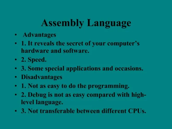
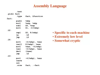
Assembly Language • True assembly is a one to one mapping with machine language instructions • Assembly language translated into object program or executable binary program • When running program, 3 levels are present, • microarchitecture • ISA • OSM
Reasons for Assembly • Pro –Faster • Pro - Smaller • Pro- Full access to hardware • interrupts • device controllers • Con- takes longer to write • Con – takes longer to debug • Con – Harder to maintain • Con – Limited to single family architecture
Why Use Assembly Language? Comparison of assembly language and high-level language programming, with and without tuning.
Assembly • Optimize code • Writing for machine with limited resources • Tuning – recoding in assembly to speed critical code sections • Understand how compilers work and what they produce • Only way to get feel of ISA level
Format of an Assembly Language Statement (1) Computation of N = I + J. (a) Pentium 4.
Format of an Assembly Language Statement (2) Computation of N = I + J. (b) Motorola 680x0.
Format of an Assembly Language Statement (3) Computation of N = I + J. (c) SPARC.
Pseudoinstructions (1) Some of the pseudoinstructions available in the Pentium 4 assembler (MASM).
Pseudoinstructions (2) Some of the pseudoinstructions available in the Pentium 4 assembler (MASM).
Macro Definition, Call, Expansion (1) Assembly language code for interchanging P and Q twice. (a) Without a macro. (b) With a macro.
Macro Definition, Call, Expansion (2) Comparison of macro calls with procedure calls.
Macros with Parameters Nearly identical sequences of statements. (a) Without a macro. (b) With a macro.
Two Pass Assemblers (1) The instruction location counter (ILC) keeps track of the address where the instructions will be loaded in memory. In this example, the statements prior to MARIA occupy 100 bytes.
Two Pass Assemblers (2) A symbol table for the program of Fig. 7-7.
Two Pass Assemblers (3) A few excerpts from the opcode table for a Pentium 4 assembler.
Pass One (1) . . . Pass one of a simple assembler.
Pass One (2) . . . . . . Pass one of a simple assembler.
Pass One (3) . . . Pass one of a simple assembler.
Pass Two (1) . . . Pass two of a simple assembler.
Pass Two (2) . . . Pass two of a simple assembler.
The Symbol Table (1) Hash coding. (a) Symbols, values, and the hash codes derived from the symbols.
The Symbol Table (2) Hash coding. (b) Eight-entry hash table with linked lists of symbols and values.
Linking and Loading Generation of an executable binary program from a collection of independently translated source procedures requires using a linker.
Tasks Performed by the Linker (1) Each module has its own address space, starting at 0.
Tasks Performed by the Linker (2) Each module has its own address space, starting at 0.
Tasks Performed by the Linker (3) Each module has its own address space, starting at 0.
Tasks Performed by the Linker (4) Each module has its own address space, starting at 0.
Tasks Performed by the Linker (5) The object modules of Fig. 7-14 after being positioned in the binary image but before being relocated and linked.
Tasks Performed by the Linker (6) The same object modules after linking and after relocation has been performed. Together they form an executable binary program, ready to run
Structure of an Object Module The internal structure of an object module produced by a translator.
Binding Time and Dynamic Relocation The relocated binary program of Fig. 7-15(b) moved up 300 addresses. Many instructions now refer to an incorrect memory address.
Dynamic Linking in MULTICS (1) Before EARTH is called.
Dynamic Linking in MULTICS (2) After EARTH has been called and linked.
Dynamic Linking in Windows Use of a DLL file by two processes.