Download

1 / 40
400 likes | 403 Vues
world. self. world. s. r. H(S) = - Σ s P(s)ln 2 P(s). H(R). if P(s 1 ,s 2 )=P(s 1 )P(s 2 ) then H(s 1 ,s 2 )=H(s 1 )+H(s 2 ). I(S,R)= Σ s,r P(s,r)ln 2 [P(s,r)/P(s)P(r)]. If r is binary , e.g. P(r=1)=a P(r=0)=1-a H(R) = a ln 2 (1/a) + (1-a) ln 2 [1/(1-a)]. θ. θ.

E N D
world self world
s r H(S) = - ΣsP(s)ln2P(s) H(R) if P(s1,s2)=P(s1)P(s2) then H(s1,s2)=H(s1)+H(s2) I(S,R)=Σs,rP(s,r)ln2[P(s,r)/P(s)P(r)]
If r is binary, e.g. P(r=1)=aP(r=0)=1-a H(R) = a ln2 (1/a) + (1-a) ln2 [1/(1-a)]
θ θ ROC curves Hits False alarms I(S,R) is further limited by the s r mapping precision s But note: ROC curves are symmetrical for ‘normal’ signals
θ ROC curves Hits False alarms ‘High-threshold’ processes lead to asymmetrical ROCs s (remember this when we discuss hippocampus and neocortex..)
If r is binary, e.g. P(r=1)=aP(r=0)=1-a H(R) = a ln2 (1/a) + (1-a) ln2 [1/(1-a)] I(S,R) is further limited by the s r mapping precision If r is linear, e.g. r = k (s + δ) (Gaussian σs, σδ) I(S,R) = ½ ln2 (1+ω2) with ω = σs / σδ(signal-to-noise)
a threshold-linear unit is limited both by its response sparsity (a) and by its signal-to-noise (ω)
Edmund Rolls’ theory of emotion dimensional reduction The Brain and Emotion, précis in Behavioral and Brain Sciences 23:177-234 (2000)
Stimulation of the amygdala produces a very high-dimensional costellation of behavioural responses…
Bull Acad Natl Med. 1998;182(7):1505-14; discussion 1515-6. Related Articles,Links [Evolution of monoamine receptors and the origin of motivational and emotional systems in vertebrates][Article in French]Vincent JD, Cardinaud B, Vernier P.IMPC, CNRS, Valbonne.The evolving vertebrate nervous system was accompanied by major gene duplication events generating novel organs and a sympathetic system. Vertebrate neural pathways synthesizing catecholamine neurotransmitters (dopamine and noradrenaline), were subsequently recruited to process increased information demands by mediating psychomotor functions such as selective attention/predictive reward and emotional drive via the activation of multiple G-protein linked catecholamine receptor subtypes. Here we show that the evolution of these receptor-mediated events were similarly driven by forces of gene duplication, at the cephalochordate/vertebrate transition. In the cephalochordate Amphioxus, a sister group to vertebrates, a single catecholamine receptor gene was found, which based on molecular phylogeny and functional analysis formed a monophyletic group with both vertebrate dopamine D1 and beta adrenergic receptor classes. In addition, the presence of dopamine but not of noradrenaline was assayed in Amphioxus. In contrast, two distinct genes homologous to jawed vertebrate dopamine D1 and beta adrenergic receptor genes were extant in representatives of the earliest craniates, lamprey and hagfish, paralleling high dopamine and noradrenaline content throughout the brain. These data suggest that a D1/beta receptor gene duplication was required to elaborate novel catecholamine psychomotor adaptive responses and that a noradrenergic system specifically emerged at the origin of vertebrate evolution.
r (t) Chemical (e.g. Peter Dayan) 106 ri (x,t) Memory (David Marr) 107 3 1 2 yrs platypus echidna DG 108 CA3 CA1 r (x,t) Metric (e.g. Joseph Atick) lizard ({ri}) Symbolic (Noam Chomsky) 109 A Simplified History of Neural Complexity infinite recursion mammalian species
Skinner box Reinforcement Learning (RL):Psychology and animal behavior literature • B. F. Skinner, 1938, The Behavior of Organisms, New York: D. Appleton-Century Publishers. • Reward strengthens likelihood of animal response. • Rats are better at learning, e.g., mazes, when they receive a reward.
Reinforcement Learning (RL)in Artificial Intelligence • The reinforcement learning (RL) problem is the problem faced by an agent that learns behavior through trial-and-error interactions with its environment. It consists of an agent that exists in an environment described by a set S of possible states, a set A of possible actions, and a reward(or punishment) rt that the agent receives each time t after it takes an action in a state. (Alternatively, the reward might not occur until after a sequence of actions have been taken.) • It is typically assumed that the environment isnon-deterministic. • Agent evaluation (in terms of rewards) may be interleaved with learning. • The objective of an RL agent is to maximize its cumulative reward received over its lifetime.
A Few Definitions • (time) step – the agent is in a state, st, takes action a, and that moves the agent to a next state, st+1. After getting to st+1 , the agent receives a reward, rt. • trial – this is the RL term used for an episode. A trial consists of a sequence of steps that terminates when either: • the agent enters a terminal/goal state, or • a predetermined time limit (number of steps) has been reached. • terminal (or absorbing) state – a state from which the agent does not leave, and which includes a final reward or punishment. A goal state is an example of a terminal state.
Markov Decision Processes(MDPs) • Unless stated otherwise, we will assume this is a Markov decision process(MDP). There are two functions, the transition function, δ(st, at) = st+1 which defines the next state given the current state and action, and the reward function, r(st, at) which provides a reward for taking this action in this state (or, alternatively, r(st)). In an MDP, δ and r depend only on the current state and action, not on earlier states or actions. If the environment is non-deterministic, then you also want to know p(st, at, st+1 ), i.e., the probability of going from st to st+1 by taking action at . All of this information combined is called a model of the environment. • The model may or may not be known to the agent. • The model may or may not be learned by the agent. The latter case is called model-free reinforcement learning. This is the type of RL that we will study.
Discount Factor • For agents with a very long (modeled as infinite) lifetime, a discount factor is useful.Future rewards are discounted. • A discount factor γ makes future rewards less valuable than current rewards. • It ensures that the total reward will converge to a finite, reasonable amount.
A “Policy” A policyis a complete mapping from every state to the action to be taken in that state. In a gridworld, we can consider a square to be a state. +1 3 obstacle -1 2 1 1 2 3 4
Objective of RL • The objective of reinforcement learning (RL) is to try to find an optimal policy. A policy, Π: S A, is a complete mapping from every state to the action to be taken in that state. • For simple problems, a policy (also called a control strategy) may be implemented as a lookup table. • An optimal policy is one that leads to optimal behavior for solving the problem, i.e., it is the policy that results in the highest cumulative reward over time. In other words, define the discounted cumulative reward achieved by policy Π from initial state st as: • Then an optimal policy is one that maximizes the discounted cumulative reward, and is defined as: PolicyΠ is followed always; 0 <= γ < 1 is a discount factor Value of a policy V*(s) is the maximum discounted cumulative reward, which is obtained by starting in state s and following Π*.
An Example of an Optimal Policy terminal states +1 3 Assumes reward is –0.04 in all non-terminal states. Rewards for terminal states (4,3) and (4,2) are shown. Assumes no discounting. obstacle -1 2 1 1 2 3 4 Note: There may be more than one optimal policy. Can you think of another optimal policy here?
An Example of Trials WhileLearning an Optimal Policy +1 +1 3 3 -1 -1 2 2 1 1 1 2 3 4 1 2 3 4 First trial Second trial Example trials on the way to learning an optimal policy: (1,1)-0.04 (2,1)-0.04 (3,1)-0.04 (3,2)-0.04 (4,2)-1 (1,1)-0.04 (1,2)-0.04 (1,3)-0.04 (2,3)-004 (3,3)-0.04 (4,3)+1 First trial Second trial
Maximum Trial Length Typically one sets a maximum number of steps per trial. The following policy gives an example why: +1 3 -1 2 1 1 2 3 4
Comment on Setting the Rewards • The choice of rewards you give the agent can determine how quickly it will learn. For example, • If you give a reward of 0.99 for every state that leads directly to the goal, and a reward of 0 for every other state, then you are giving a great deal of prior knowledge to your agent, and it can learn very fast because little learning is required. In essence, you areteaching the agent how to get to the goal by carefully selecting your rewards. • If you give relatively equal rewards (e.g., close to 0) from all states other than the terminal states, it will take the agent a long time to learn. The previous two slides give an example of this. • For your projects, you probably want to do something in the middle of these two extremes.
Temporal Difference (TD) Learning (Sutton, 1984) • The objective is to learn an estimate of the utility of all states. The utility is the expected sum of rewards from this state on, i.e., it is a measure of V*(s). • Once the agent has learned an estimated utility for each state, it can use this utility for deciding which action to take next – it will choose the action that leads to the next state with the highest utility.
Temporal Difference Learning • The objective is to learn an estimate of the utility of all states. The utility is the expected sum of rewards from this state on. • Key idea: Use insight from dynamic programming to adjust the utility of a state based on the immediate reward and the utility of the next state. • U(s) U(s) + α(r(s) + γU(s’) – U(s)) the observed successor state reward obtained in state i learning rate Essence: (1- α)*(old) + α*(new) U(s) is an estimate of V*(s), which is the maximum discounted cumulative reward starting in state s.
A Simple TD Learning Algorithm • Initialize U(s) = 0 for all non-terminal states s. For terminal states, U(s) = r(s). Start in a designated initial state s0. (We assume all other states are reachable from s0.) • For each transition δ(s, a) = s’ and reward r(s) for going from state s to state s’, do: • U(s) U(s) +α(r(s) + U(s’) – U(s)) • Repeat above step until the difference in successive values (before/after update) of U is less than or equal to some small desired ε (called convergence).
Active learning in an unknown environment • The TD learner just described is a passive learner, i.e., a learner that observes the state and reward sequences and estimates the expected sum of rewards in all non-terminal states that it visits. After learning the utilities, actions can be chosen based on those utilities. • An active learner must consider what actions to take, what their outcomes may be, and how they affect the rewards achieved. An active learner takes actions while it learns. Only an active learner can handle a dynamic environment.
Active learning s1,a1,r1,learn, s2,a2,r2,learn,………. Here, the reward is a function of the state and action, i.e., ri (si, ai).
Interaction between world and an active learning robot • World: you are in state 34. You have three possible actions from this state. • Robot: I’ll take action 2. • World: you are in state 77. Your immediate reward is –7. You have two possible actions from this state. • Robot: I’ll take action 1. • World: you are in state 34. Your immediate reward is 3. You have three possible actions from this state. • …………
Objective of Q-Learning Let Q*(s, a) be the maximum, discounted, cumulative reward for taking action a in state s, and then continuing to choose actions optimally (according toΠ*). This is analogous to V*(s), the maximum discounted cumulative reward, which is obtained by starting in state s and following Π*(s). Note that: Assume δ(s, a) = s’.Then Q*(s, a) can be defined recursively as: Objective:Learn Q(s, a), which estimates Q*(s, a). Note that â is a variable here where
Q-Learning Update Formula • Learn an action value function Q mapping state-action pairs to the expected utility of the sequence starting with that state/action pair. There is no need to learn the functions δ(s, a) or r(s, a), or p(s, a, s’), i.e., the model of the environment. • The procedure UPDATE-Q-VALUE(s, a) is: • The Q-value is related to the utility value U by: Recall from previous slide:
RL needs signal that Respond to affective contingencies Affect learning of predictions and actions Are essentially scalar Broadcast their information multimodally Neuromodulators in fact Respond to reinforcers and surprise Are known to affect synaptic plasticity Come from small mid-brain nuclei Have extensive arborization throughout the brain As for the Neural ImplementationPeter Dayan notes that…