Download
1 / 51
520 likes | 636 Vues
B. A. B. B. A. A. x. x. x. VSP Multiple Interferometry. 3x3 Classification Matrix. SSP. VSP. SWP. SSP. SSP. SSP. SSP. VSP. SSP. SWP. VSP. VSP. SSP. VSP. VSP. VSP. SWP. SSP. SWP. SWP. SWP. VSP. SWP. SWP. Interferometry Summary. G( A | x )*. G( B | x ).

E N D
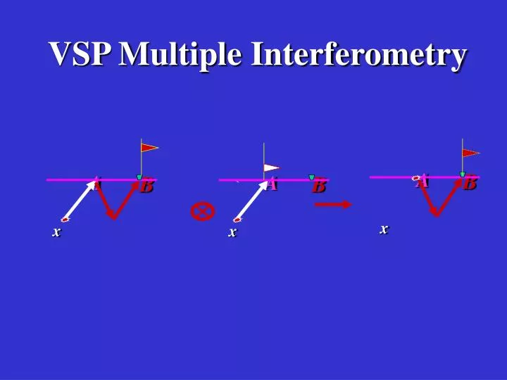
B A B B A A x x x VSP Multiple Interferometry
3x3 Classification Matrix SSP VSP SWP SSP SSP SSP SSP VSP SSP SWP VSP VSP SSP VSP VSP VSP SWP SSP SWP SWP SWP VSP SWP SWP
Interferometry Summary G(A|x)* G(B|x) = G(A|B) x B A B B A A x x x ! k Key Point #1: Common Raypath Cancels Key Point #2: Every Bounce Pt on Surface Acts a New Virtual Source Key Point #3: Summation over Sources Picks out Specular Contribution Key Point #4: Kills Source Statics and no need to know src location or excitation time Key Point #5: Huge increase in Illumination Area
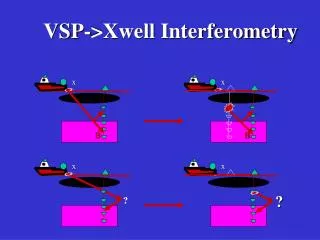
G(A|x)* G(B|x) = G(A|B) x Correlation Redatuming VSP ->SSP ! k Standard VSP Primary VSP -> SSP
Reciprocity Correlation Equation Given: VSP data G(A|x) Find: SSP data G(A|B) B A x
o o S o S well S Reciprocity Correlation Equation Given: VSP data G(A|x) Find: SSP data G(A|B) A B x
n { } * * * S + S + S - G(A|x) = G(A|B) - G(B|A) G(B|x) G(A|x) G(B|x) x o k o o o o G(A|x)* G(B|x) = Im[G(A|B)] well 2 d x S o S well S Reciprocity Correlation Equation Given: VSP data G(A|x) Find: SSP data G(A|B) A B x
x k G(A|x)* G(B|x) = Im[G(A|B)] G(B|A) A B A B A B x x x Reciprocity Correlation Equation VSP => SSP Given: VSP data G(A|x) Find: SSP data G(A|B) G(A|x) G(B|x)*
Examples 1. 2D Synthetic VSP Data 2. 2D Field VSP Data 3. 3D VSP Data
Well 256 Sources V = 1.5 - 3.0 km/s 0 Depth (km) SEG/EAGE Model 2 0 X (km) 3
Acquisition Parameters: Well location: (1.5 km, 0 km) Source interval: 10 m Source number: 256 Receiver interval: 10 m Receiver depth range: 0.1 -1 km Receiver number: 91 Sample interval: 1 ms Recording length: 3 s Well 0 1 km Depth (km) 2 0 X (km) 3
VSP VSP SSP 1. FK Filter up and downgoing waves x x k G(A|x)* G(B|x) G(A|x)* = Im[G(A|B)] G(B|x) 2. Correlation: f(A,B,x) = f(A,B,x) 3. Summation: k = Im[G(A|B)] M(x) = Mig(G(A|B)) 4. Migration: A B A B A B x x x Implementation
Depth (km) 0.2 0.9 0 CSG 160 Time (s) 3
Depth (km) 0.2 0.9 0 Ghosts (CSG 160) Time (s) 3
X (km) 1.4 2.4 Xcross 60 X (km) 0 2.4 0 Time (s) CRG 60 3
Xcorr Mig (45) Xcorr. Mig(15’) Kirchh Mig (45) 0.5 Depth (km) 2.0 0.5 2.5 0.5 2.5 0.5 2.5 X (km)
0 Well Depth (m) 900 50 Raw Data Static errors (ms) -50 Static Errors at Well
Kirchhoff Migration Static Error: 25 ms Static Error: 50ms 2.5 X (km) Static Error: 0 0.5 Depth (km) 2.0 0.5 2.5 0.5 2.5 0.5
Lesson: Immune to statics at well Crosscorrelation Migration Static Error: 25ms Static Error: 50 ms 2.5 X (km) Static Error: 0 0.5 Depth (km) 2.0 0.5 2.5 0.5 2.5 0.5
Velocity Model Well X (m) 925 0 0 V (m/s) 4000 Depth (m) 1900 1300 Shots: 92; Receivers: 91 (50m -950 m)
CSG 51 Ghost Component 0 S A Time (s) Well G X 3 50 950m 50 950m
CSG 51 Primary Component 0 Time (s) S A Well G X 3 50 950m 50 950m
8 Receivers Lesson: Super-illumination Primary 1st-order multiple 0 Depth (m) 1300 X (m) 0 0 X (m) 925 925
Examples 1. 2D Synthetic VSP Data 2. 2D Field VSP Data:Friendswood Data 3. 3D VSP Data
Depth (ft) 30 900 0 Raw Data(CRG15) Time (s) 0.3
Depth (ft) 30 900 0 Ghosts Time (s) 0.3
Field Data (CSG 25) Trace No. 5 24 xcorr data (muted) 0.2 Time (s) 1.2 Master trace Master trace Trace No. 5 24 0.5 Raw data (muted) Time (s) 1.4
X (ft) X (ft) 0 400 0 400 200 Standard mig Xcorr. mig Depth (ft) 1300
Well data Xcorr. Exxon Data Standard 0 Depth (ft) 1100
Examples 1. 2D Synthetic VSP Data 2. 2D Field VSP Data:Middle East Data 3. 3D VSP Data
A Real Walkaway VSP Experiment 0 401 shots on a topographic surface well Depth (m) 1400 12 geophones at ~ 1400 - 1500 m depth 1500 0 10000 Offset (m)
A Common Receiver Gather 0.4 Time (s) 1.8 0 10000 Offset (m)
Work flow Separate up and down going wavefields Upgoing wavefield Downgoing wavefield Statics Statics Statics Ray tracing Pick first-break Specular interferometry Primaries migration Multiples migration
Standard vs Interferometry Mig VSP (Narrow vs Wide Illumination) VSP Interferometry Imaging 1500 m VSP Primaries migration 1000 m 500 m 100 Time (ms) geophones 1600
Examples 1. 2D Synthetic VSP Data 2. 2D Field VSP Data: GOM Data 3. 3D VSP Data
VSP Multiple (12 receivers 13 kft @ 30 ft spacing; 500 shots) 5000 Depth (ft) 13000 X (ft) 0 56000 TLE, Jiang et al., 2005
Surface Seismic 5000 Depth (ft) 13000 X (ft) 0 56000 TLE, Jiang et al., 2005
VSP Multiple (12 receivers 13 kft @ 30 ft spacing; 500 shots) 5000 Depth (ft) 13000 X (ft) 0 56000 TLE, Jiang et al., 2005
Examples 1. 2D Synthetic VSP Data 2. 2D Field VSP Data: GOM Data 3. 3D VSP Data: Synthetic
3D SEG Salt Model Test (He, 2006)
VSP Multiples Migration Stack of 6 receiver gathers ( Courtesy of P/GSI: ~¼ million traces, ~3 GB memory, ~4 hours on a PC ) (He, 2006)
Examples 1. 2D Synthetic VSP Data 2. 2D Field VSP Data: GOM Data 3. 3D VSP Data: GOM BP Data
Survey Geometry ~ 11 km ~ 11 km 3 similar spirals, each corresponding to an offset-ed geophone group. Each geophone group has 12 geophones. ~ 5 km deep
3D WEIM Result Migration of only one receiver gather
Why was the 2D mirror migration good out to 50,000 feet offset? Slice of 3D WEIM Result
VSP->SSP Summary G(A|x)* G(B|x) = G(A|B) x B A B B A A x x x ! k Key Point #1: Common Raypath Cancels Key Point #2: Every Bounce Pt on Surface Acts a New Virtual Source Key Point #3: Summation over Sources Picks out Specular Contribution Key Point #4: Kills Source Statics and no need to know src location or excitation time Key Point #5: Huge increase in Illumination Area
VSP->SSP Caveats G(A|x)* G(B|x) = G(A|B) x B A B B A A x x x ! k 1. Infinitely source wide aperture. Artifacts must be recognized/fixed) 2. No attenuation assumed (remedy: attenuation compensation) 3. Be careful beneath salt domes (extra bounces get double defocused by salt). 3. Violation of assumptions seems ok for kinematics, not amplitudes