Download
1 / 30
300 likes | 456 Vues
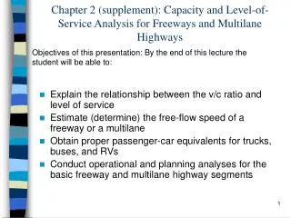
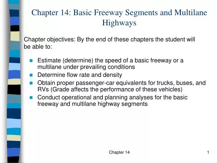
Chapter 14: Basic Freeway Segments and Multilane Highways. Chapter objectives: By the end of these chapters the student will be able to:. Estimate (determine) the speed of a basic freeway or a multilane under prevailing conditions Determine flow rate and density

E N D
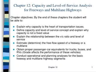
Chapter 14: Basic Freeway Segments and Multilane Highways Chapter objectives: By the end of these chapters the student will be able to: • Estimate (determine) the speed of a basic freeway or a multilane under prevailing conditions • Determine flow rate and density • Obtain proper passenger-car equivalents for trucks, buses, and RVs (Grade affects the performance of these vehicles) • Conduct operational and planning analyses for the basic freeway and multilane highway segments Chapter 14
14.1 Facility Types Chapter 14
14.2 Basic freeway and multilane highway characteristics Basic freeway segments: Segments of the freeway that are outside of the influence area of ramps or weaving areas. Chapter 14
14.2.1 Basic freeway and multilane highway characteristics (This is Figure 14.2 for basic freeway segments) Chapter 14
14.2.1 continued Chapter 14
Fig 14.3 Base Speed-Flow Curves for Multilane Highways (For multilane highways) Chapter 14
Fig 14.3 Base Speed-Flow Curves for Multilane Highways Chapter 14
14.2.2 Level of Service www.utahcommuterlink.com LOS B LOS C or D LOS A LOS E or F Chapter 14
14.2.3 Service flow rates and capacity Chapter 14
14.3 Analysis methodologies Most capacity analysis models include the determination of capacity under ideal roadway, traffic, and control conditions, that is, after having taken into account adjustments for prevailing conditions. Basic freeway segments Chapter 14
Prevailing condition types considered (p.291): • Lane width • Lateral clearances • Type of median (multilane highways) • Frequency of interchanges (freeways) or access points (multilane highways) • Presence of heavy vehicles in the traffic stream • Driver populations dominated by occasional or unfamiliar users of a facility Chapter 14
Factors affecting: examples Trucks occupy more space: length and gap Drivers shy away from concrete barriers Chapter 14
14.3.1 Types of analysis • Operational analysis (Determine speed and flow rate, then density and LOS) • Service flow rate and service volume analysis (for desired LOS) MSF = Max service flow rate • Design analysis (Find the number of lanes needed to serve desired MSF) Chapter 14
Service flow rates vs. service volumes What is used for analysis is service flow rate. The actual number of vehicles that can be served during one peak hour is service volume. This reflects the peaking characteristic of traffic flow. Stable flow SFE Unstable flow E F Flow D SVi = SFi * PHF C SFA Congested B A Uncongested Density Chapter 14
Sample operational analysis 1800 pc/h/ln FFS=65 mph S = 65 - 0.00001418 (1800 – 1400)2 = 62.7 mph Chapter 14
14.3.2 (cont.) Adjustment to free-flow speed on a freeway TRD = Total number of on- and off-ramps within ±3 miles of the midpoint of the study segment, divided by 6 miles. Chapter 14
Read p.294 right column carefully. 14.3.2 (cont.) Adjustment to free-flow speed on a multilane highway BFFSi: Read p.294 left column, bottom (and slide #16). fLW: use Table 14.5 Chapter 14
Choosing a free-flow speed curve (p.296) Not recommended to interpolate. So, this table was given. This table is for both freeways and multilane highways. Chapter 14
Examples for determining FFSs Chapter 14
14.3.3 Determining the heavy-vehicle factor PP = percent passenger cars PT = percent trucks & buses PR = percent recreational vehicles (RVs) ET = PCE for trucks and buses ER = PCE for RVs Grade and slope length affects the values of ET and ER. Chapter 14
How we deal with long, sustaining grades… (p.298) There are 3 ways to deal with long, sustaining grades: extended general freeway segments, specific upgrades, and specificdowngrades. (1) Extended segments: where no one grade of 3% or greater is longer than ¼ mi or where no one grade of less than 3% is longer than ½ mi. And for planning analysis. (p.298, left column) Chapter 14
How we deal with long, sustaining grades…(cont) (2) Specific upgrades: Any freeway grade of more than ½ mi for grades less than 3% or ¼ mi for grades of 3% or more. (For a composite grade, refer to page 299 right column.) Use the tables for ETand ER for specific grades. • (3) Specific downgrades: • If the downgrade is not severe enough to cause trucks to shift into low gear, treat it as a level terrain segment, ET = 1.5. • Otherwise, use the table for downgrade ET • For RVs, downgrades may be treated as level terrain, ER = 1.2. Chapter 14
Tables for PCE for specific grades When using these look-up tables, care must be taken to observe the boundary condition. Upper boundaries are “Closed” in these tables. Chapter 14
Example for using specific grades Chapter 14
Average grade or composite grade? (p.299) • In a basic freeway segment analysis, an overall average grade can be substituted for a series of grades if no single portion of the grade issteeper than 4% or the total length of the grade is less than 4,000 ft. (See the example in p.300 right column.) • For grades outside these limits, the composite grade procedure is recommended. The composite grade procedure is used to determine an equivalent grade that will result in the same final truck speed as used to determine an equivalent grade that will result in the same final truck speed as would a series of varying grades. (page 301-302: read these pages carefully for strength and weakness of this method) • For analysis purposes, the impact of a grade is worst at the end of its steepest (uphill) section. (e.g. if 4000 ft of 4% grade were followed by 1000 ft of 3% grade, passenger-car equivalents would be found for a 4000 ft, 4%. Chapter-end Problem 14-3(c) is this case.) But, what if 1000 ft of 4% and 1000 ft of 3%? Chapter 14
Composite grade (Read p.302 for explanation of the steps.) 3% grade 3000 ft followed by 5% grade 5000 ft Find the equivalent (composite) grade. Chapter 14
14.3.4 Determining the driver population factor • Not well established • Between a value of 1.00 for commuters to 0.85 as a lower limit for other driver populations • Usually 1.00 • If there are many unfamiliar drivers use a value between 1.00 and 0.85 • For a future situation 0.85 is suggested Chapter 14
Planning analysis (or design analysis) You want to find out how many lanes are needed for the targeted level of service. Step 1: Find fHV using for ET and ER. Step 2: Try 2 lanes in each direction, unless it is obvious that more lanes will be needed. Step 3: Convert volume (vph) to flow rate (pcphpl), vp, for the current number of lanes in each direction. Step 4: If vp exceeds capacity, add one lane in each direction and return to Step 2. Step 5: Compute FFS. Step 6: Determine the LOS for the freeway with the current number of lanes being considered. If the LOS is not good enough, add another lane and return to Step 3. See Example 14-7 Chapter 14
14.4 Sample Problems • We will review the manual method and HCS2010 on Friday. 14.5 Calibration issues I recommend you to read it. It will be helpful when you want to use local values (Remember HCS values are national average values). Chapter 14