Application of Nonlinear Two Dimension Wave Equation Dual Reciprocity Boundary Element Method

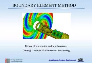
1. International Research Research and Development (IJTSRD) International Open Access Journal International Open Access Journal International Journal of Trend in Scientific Scientific (IJTSRD) ISSN No: 2456 ISSN No: 2456 - 6470 | www.ijtsrd.com | Volume Application of Nonlinear Two-Dimension Wave Equation Dual Dimension Wave Equation Dual 6470 | www.ijtsrd.com | Volume - 2 | Issue – 3 Application of Nonlinear Two Reciprocity Boundary Element Method Reciprocity Boundary Element Method Reciprocity Boundary Element Method P. Parameshwari G. Pushpalatha Pushpalatha Department of Mathematics, Vivekanandha College of Arts and Sciences for , Tiruchengode, Namakkal, Tamil Nadu, India Research Scholar, Department of Mathematics, Vivekanandha college of Arts and Sciences for Women, Tiruchengode, Namakkal, Tamil N , Tiruchengode, Namakkal, Tamil Nadu, India Research Scholar, Department of Mathematics, Vivekanandha college of Arts and Sciences for Assistant Professor, Department of Mathematics, Vivekanandha College of Arts and Sciences for Women, Tiruchengode, Namakkal, T ABSTRACT The constructive numerical implementation of the two-dimensional dual boundary element method. This paper present to solve nonlinear 2 equation defined over a rectangular spatial domain the boundary conditions. Two-dimension wave equation is a time-domain problem, with three independent variables u,v,t. The applied to 2-D wave equation satisfactory authority. Keywords: 2D non-linear wave equation, analysis, acoustics, dynamics, boundary element method acoustics, dynamics, boundary element method Where ?? belongs to a certain class of linear operators, functions ???ℎ and f are assumed to be continuous. The constructive numerical implementation of the dual boundary element method. This paper present to solve nonlinear 2-D wave equation defined over a rectangular spatial domain the belongs to a certain class of linear and f are assumed to be The laplace transform of the nth order equation with The laplace transform of the nth order equation with respect to t gives dimension wave equation domain problem, with three independent D wave equation ??[W(u,v,k)] ???? ????? linear wave equation, analysis, ≡??????ℎ(u,v) ???U (u,v,k) = F(u,v,k) + B (u,v,k) The Laplace Transform: The laplace transform in solving ordinary and partial differential equations. In this present work to eliminate the time-dependency to product a subsidiary equation is then solved in complex arithmetic by DRBEM. Let f be a function of t. The laplace transform of f is defined as follows transform in solving ordinary and partial differential equations. In this present work to dependency to product a subsidiary equation is then solved in complex arithmetic by DRBEM. Let f be a function of t. The laplace Where W(u,v,k) is the laplace transform of w(u,v,t) with respect to t, F is the laplace transform of f and B containsall the initial condition information. Equation (n-h)th order equation only u and v which has to be solved for W(u,v,k) over the domain c subject to the transformed boundary conditions for particular values of the complex variable k. The boundary conditions for equation taking the Laplace transform with respect to t of the boundary condition. respect to t of the boundary condition. Where W(u,v,k) is the laplace transform of w(u,v,t) with respect to t, F is the laplace transform of f and B containsall the initial condition information. Equation h)th order equation only u and v which has to be the domain c subject to the transformed boundary conditions for particular values of the complex variable k. The boundary conditions for equation taking the Laplace transform with ∞ ? F(g) = ∫ ???? f(t)dt When the laplace transform exists, it is denoted by {f(t)}. When the laplace transform exists, it is denoted by Numerical Inversion of the Laplace Numerical Inversion of the Laplace Transforms: Consider the nth order linear PDF in just two independent spatial variables u,v and time t, with coefficients independent of time, defined for t > 0 over the finite region D∈??, with sufficient initial and boundary conditions the unique solution w (u,v,t) to the problem. This function represented as follows the problem. This function represented as follows Consider the nth order linear PDF in just two independent spatial variables u,v and time t, with coefficients independent of time, defined for t > 0 Analytic inversion of the laplace transform is defined as a contour integration in the complex plane. The Bromwich contour is commonly chosen. The inversion formula for the laplace transform is as Analytic inversion of the laplace transform is defined as a contour integration in the complex plane. The Bromwich contour is commonly chosen. The inversion formula for the laplace transform is as follows , with sufficient initial and boundary conditions the unique solution w (u,v,t) to Where c is a suitable complex number, k is a real Where c is a suitable complex number, k is a real V(t)=(2?z)^-1 ?????ℎ? ????????ℎ ??[w(u,v,t)] ≡????ℎ(u,v) = f (u,v,t) @ IJTSRD | Available Online @ www.ijtsrd.com @ IJTSRD | Available Online @ www.ijtsrd.com | Volume – 2 | Issue – 3 | Mar-Apr 2018 Apr 2018 Page: 2041

2. International Journal of Trend in Scientific Research and Development (IJTSRD) ISSN: 2456-6470 nonnegative parameter and v(k) must be analytic in the right-half plane of the complex plane. The Use of Dual Reciprocity Boundary Element Method: This method is based on the numerical evaluation of the Bromwich integral. Salzers method is in fact Gussian quadrature of the Bromwich integral and gives the following approximation to v(t) The general form of equation as the follows ∇?W-??W = f(u,v) Where ?? includes the coefficients of all the W dependent terms and f(u,v) represents the remaining terms. The source term is then transferred to the boundary by using dual reciprocity principles. So the interpolation approximation is needed only for source term f(u,v). A brief description of the DRM is given next. V(t)≈ v(t)=???????(??/t)^? v(??/t) Where ?? and ?? are the abscissa and weights of the Gaussian quadrature formula of order p. The values of ?? and ?? are tabulated for various values of ?. It is possible to compute W(u,v,k) the equation numerical approaches with its transformed boundary conditions for a fixed value of the complex parameter s. The approximate solution v(t) is now obtained from the p values of V(??/t). The value of V(??/t) can be identified with W(u,v,??/t), the solution of equation s = ??/t. For each value of t,for N times. Dual Reciprocity Method: Consider a set of M collocation points arbitrarily located in the domain σ the function f may be approximated by the following expression: ? ??? F(u,v) = ∑ (u,v) ?? ?? Where M is sum of E boundary notes and L interior(DRM) notes subcribs c denotes any interpolation node include boundary and DRM notes ?? and ?? are interpolation coefficients and radial basis function (RBF)respectively. The functions such as polynomial can be seleced as ??(for2D): Governing Equation and Boundary Conditions: Wave equation is a time-space dependent problem. General 3-D wave equation is as follows: ??? ??? = ??∇?w = ??(??? ???+??? ???), ?+??? ??(u,v) = 1+??(u,v)-?????? (u,v)∈??,t ∈ (0,∞) ?? For which w(u,v,t) is the unknown solution and ∇? the Laplacian and c is a constant speed of the wave propagation, we assume to be constant in the whole environment.We adopt the unit square (u,v) ∈ [0,2]×[0,2] as the spatial solution domain with 200 elements per each side and 200 interior points, c = 2,with initial condition w(u,v,0) = sin(??) × sin(??) Where ??(u,v) = ?(? − ??)?+ (? − ??)?. The inverse of matrix ψ, determined vector ? ⃗. ????? ??? ??=∑ ??? Reference 1)Katsikadelis, J. T. Boundary element, theory and application Elsevier publication,2002. 2)Aliabadi, M.H., and Wen, P.H. Boundary Element Methods in Engineering and sciences, Imperical College press, 2011. 3)Salzer, H.E. “Orthogonal polynomials arising in the numerical evaluation of inverse Laplace transforms,” M.T.A.C. 9, 164-177, 1955. 4)Pozrikidis, C. A practical guide to boundary element methods with the software library BEMLIB, Chapman & Hall/CRC,2002. 5)Narayanan, G. V. and Beskos, D. E. Numerical operational methods for time dependent linear problems, International journal of numerical Methods in Engineering, 18, 1829-1854, 1982. ?? ??(u,v,0) and w = 0 on the boundaries. The analytical solution of equation W(u,v,t) = cos(√2??) × sin(??) × sin(??) Taking the laplace transform with respect to t converts the subsidiary equation as follows ??? ???+??? ???- ??W = -k× sin(??) × sin(??) The subsidiary equation will be solved using DRBEM. The next section describes this equation. @ IJTSRD | Available Online @ www.ijtsrd.com | Volume – 2 | Issue – 3 | Mar-Apr 2018 Page: 2042