Download
1 / 97
1.1k likes | 1.51k Vues
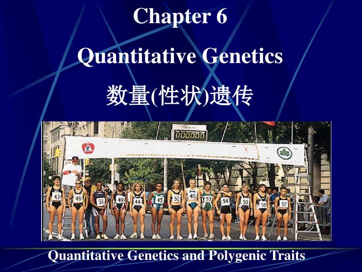
Chapter 6 Quantitative Genetics 数量 ( 性状 ) 遗传. Quantitative Genetics and Polygenic Traits. 1914 Class of the Connecticut Agricultural College (fig. 13.17 from text).

E N D
Chapter 6 Quantitative Genetics 数量(性状)遗传 Quantitative Genetics and Polygenic Traits
1914 Class of the Connecticut Agricultural College (fig. 13.17 from text) Phenotypic variation in quantitative traits often approximates a bell-shaped curve: thenormal distribution!Example: distribution of height in humans
Quantitative Inheritance • Analysis of Polygenic Traits • Heritability (遗传力\遗传率) • Mapping Quantitative Trait
6.1 Quantitative Inheritance The Multiple-Factor HypothesisAdditive Alleles: The Basis of Continuous Variation Calculating the Number of Genes The Significance of Polygenic Inheritance • 6.2 Analysis of Polygenic Traits The Mean Variance Standard Deviation Standard Error of the Mean Analysis of a Quantitative Character
6.3 Heritability Broad-Sense HeritabilityNarrow-Sense HeritabilityArtificial SelectionTwin Studies in Humans • 6.4 Mapping Quantitative Trait Loci
Trait that exhibit quantitative phenotypic variation are often under the genetic control of alleles whose influence is additive(累加/加性) in nature, resulting in continuous variation. • Such trait can be analyzed and characterized using statistical methods, which also allow the assessment of the relative importance of genetic factors during phenotypic expression. • Such calculation establish the heritability of traits in a population. In humans, twin studies provide a similar, but less precise, estimate. • Recently developed techniques allow the localization within the genome of loci contributing to quantitative traits.
Previous chapters: Up to now, we have focused on genetics of: Qualitative traits – genetic variants fall into discrete, easily detectable classes. phenotypic variation classified into distinct traits, e.g. 1. Seed shape in peas (round or wrinkled) ,pea plant tall and dwarf , 2. Eye color in fruit flyDrosophila (red or white) 3. Blood types in humans (A, B, AB, or O) 4. squash shape spherical, disc-shaped and elongated, • These phenotypes exemplifies discontinuous variation
But what about: Quantitative traits – phenotypic variationcontinuous, and individuals do not fall into discrete classes. Example: Height in humans • Many other traits in a population demonstrate fairly more variation and are not easily categorized into distinct classes. For Example: Some Plant Disease Resistances Weight Gain in Animals , Fat Content of Meat IQ , Learning Ability , Blood Pressure
Quantitative Characteristics Definitions • In natural populations, variation in a character takes the form of a continuous phenotypic range rather than discrete phenotypic classes. • In other words, the variation is quantitative, not qualitative . • Mendelian genetic analysis is extremely difficult to apply to such continuous phenotypic distributions, so statistical techniques are employed instead.
Many traits are influenced by the combined action of many genes and are characterized by continuous variation. These are called polygenic traits. Continuously variable characteristics that are both polygenic and influenced by environmental factors are called multifactorial traits. Examples of quantitative characteristics are height, intelligence & hair color. Quantitative Characteristics
Discontinuous traits–qualitative traits with only a few possible phenotypes that fall into discrete classes; phenotype is controlled by one or only a few genes (ex.: tall or short pea plants; red, pink or white snapdragon flowers) 质量性状——变异不连续的 • Continuous traits -Quantitative trait do not fall into discrete classes; a segregating population will show a continuous distribution of phenotypes - more common term for continuous trait; a trait that has a quantitative value (yield, IQ) 数量性状——变异连续的 • Quantitative Genetics - the field of genetics that studies quantitative traits
基本物质为呈连续分布的数量性状,而表型性状则为不连续分布的质性状。基本物质为呈连续分布的数量性状,而表型性状则为不连续分布的质性状。 • 基本物质处于某一特定范围内,表现为正常,如果超出某一阈值,表型就不正常,如血压,血糖含量,抗病力等。 • 基本物质受多基因控制,但性状的改变仅发生在基本物质达到或者超过某一阈值时才发生。所以多基因控制的性状,也可以表现为非此即彼,全或无的表型。 Threshold(阈值)model
Quantitative (discontinuous)traits are controlled by multiple genes, each segregating according to Mendel's laws. • These traits can also be affected by the environment to varying degrees.
1、Quantitative Inheritance • A major task of quantitative genetics is to determine the ways in which genes interact with the environment to contribute to the formation of a given quantitative trait distribution.
At the beginning of the 20th century, geneticists noted that many characters in different species had similar patterns of inheritance, • such as height and stature in humans, • seed size in the broad bean, • grain color in wheat, and • kernel number and ear length in corn. • In each case, offspring in the succeeding generation seemed to be a blend of their parents' characteristics.
What is the genetic and environmental contribution to the phenotype? • How many genes influence the trait? • Are the contributions of the genes equal? • How do alleles at different loci interact: additively? epistatically? • How rapid will the trait change under selection?
What is the genetic basis of variation in quantitative traits? Characteristics of Quantitative Traits 1. Polygenic – affected by genetic variation at many different gene loci. 2. Phenotypic effects of allelic substitution are usually small and additive. • Each allelic substitution results in an incremental change in overall phenotype. 3. Phenotypic variation in quantitative traits usually influenced by environmental variation as well as by genetic variation.
The Multiple Factor Hypothesis Polygeic Traits • tabaco plants in a cultivated field or wild at the side of the road are not neatly sorted into categories of "tall" and "short," (Figure 6-1).
The issue of whether continuous variation could be accounted for in Mendelian terms caused considerable controversy in the early 1900s. • William Bateson and Gudny Yule, who adhered to the Mendelian explanation of inheritance, suggested that a large number of factors or genes could account for the observed patterns. • This proposal, called the multiple-factor hypothesis, implied that many factors or genes contribute to the phenotype in a cumulative or quantitative way. • However, other geneticists argued that Mendel's unit factors could not account for the blending of parental phenotypes characteristic of these patterns of inheritance and were thus skeptical of these ideas.
NB - no nice 3:1, 9:3:3:1 ratios! This is the normal type of result for most traits. Due to:- 1. Multiple genes each having some cumulative effect on the phenotype - (QTL’S) plus 2. Environmentally caused variation By 1920, the conclusions of several critical sets of experiments largely resolved the controversy and demonstrated that Mendelian factors could account for continuous variation. In one experiment, Edward M. East crossed two strains of the tobacco plant Nicotiana longiflora.
Additive alleles:The Basis of Continuous variation • The multiple-factor hypothesis, suggested by the observations of East and others. embodies the following major points: l. Characters that exhibit continuous variation can usually be quantified by measuring, weighing, counting, and so on 2. Two or more pairs of genes, located throughout the genome, account for the hereditary influence on the phenotype in an additive way. Because many genes can be involved, inheritance of this type is often called polygenic.
3. Each gene locus may be occupied by either an additive allele, which contributes a set amount to the phenotype,or by a non additive allele, which does not contribute quantitatively to the phenotype. 4. The total effect on the phenotype of each additive allele, while small, is approximately equivalent to all other additive alleles at other gene sites. 5. Together the genes controlling a single character produce substantial phenotypic variation. 6. Analysis of polygenic traits requires the study of large numbers of progeny from a population of organisms.
These points center around the concept that additive alleles at numerous loci control quantitative traits. To illustrate this, let's examine Herman Nilsson-Ehle's experiments involving grain color in wheat performed In one set of experiments, wheat with red grain was crossed to wheat with white grain (Figure 6-3).
P Nilsson-Ehle’s crosses demonstrated that the difference between the inheritance of genes influencing quantitative characteristics and the inheritance of genes influencing discontinuous characteristics is the number of loci that determine the characteristic. Both quantitative (continuous) and discontinuous traits are inherited according to Mendel’s laws. F1 F2
Three genes act additively to determine seed color. • The dominant allele of each gene adds an equal amount of redness; the recessive allele adds no color to the seed. • A adds 1 unit of redness, a does not. • B adds 1 unit of redness, b does not. • C adds 1 unit of redness, c does not.
As the number of polymorphic loci increases, phenotypic variation approaches a continuous normal distribution! As the number of loci affecting the trait increases, the # phenotypic categories increases. Number of phenotypic categories = (# gene pairs × 2) +1 Connecting the points of a frequency distribution creates a bell-shaped curve called a normal distribution.
0.18 Ten 0.16 Polymorphic Loci 0.14 0.12 0.10 Proportion of Individuals 0.08 0.06 0.04 0.02 0.00 0 -10 -8 -6 -4 -2 +2 +4 +6 +8 +10 Relative Height (Deviation from Mean) 2. Additional phenotypic variation introduced by environmental variation will further blur distinctions between genotypic classes!
Calculating the Number of Genes When additive effects control polygenic traits, it is of interest to determine the number of genes involved. If the ratio (proportion) of F2 individuals resembling either of the two most extreme phenotypes (the parental phenotypes) can be determined, then the number of gene pairs involved (n) can be calculated using the following simple formula: 1/4n=ratio of F2 individuals expressing either extreme phenotype
Table 6.1 lists the ratios and number of F2 phenotypic classes produced in crosses involving up to five gene pairs. For low numbers of gene pairs, it is sometimes easier to use the (2n + 1) rule. When n = 2. 2n + 1 = 5. That is, each phenotypic category can have 4. 3, 2, 1, or 0 additive alleles. When n = 3. 3n + 1 =7, and each phenotypic category can have 6, 5, 4, 3, 2, 1, or 0 additive alleles, and so on.
Calculation of Ratio of F2 with a Given Genotype • For example, you are asked what proportion of the F2 generation of a cross between a dark red and a white-seeded wheat plant would have two dominant alleles. • Aassuming 2 loci, this would include the following phenotypes: • AaBb (1/2 x 1/2 = 1/4 or 4/16)AAbb (1/4 x 1/4 = 1/16) • Isolate each gene and determine the proportion of each class (product law), then add the three together (sum law). Final answer = 6/16 aaBB (1/4 x 1/4 = 1/16)
Corn Height Model: minimal height = 32” 4 dominant alleles interact equally and additively A adds 8” to height, a does not B adds 8” to height, b does not C adds 8” to height, c does not D adds 8” to height, d does not e.g. AABbCcDd = 32 + (5 × 8) = 72” tall
Strain 1 AABBccdd (64”) Strain 2 aabbCCDD (64”) P [32 + (4x8)] F1 AaBbCcDd (64”) F2 a continuous distribution from aabbccdd (32”) to AABBCCDD (96”) 16 × 16 Punnett square
The number of genes involved is n, where the ratio of F2 individuals expressing either extreme phenotype is 1/4n. The number of genes involved is n, where the ratio of F2 individuals expressing either extreme phenotype is 1/4n. In this case 1 out of 256 is minimum height, therefore the number of genes involved is 4 (44=256). In this case 1 out of 256 is minimum height, therefore the number of genes involved is 4 (44=256).
The significance of Polygenic Inheritance • Polygenic inheritance Is a significant concept because it appears to serve as the genetic basis for a vast number of traits involved in animal breeding and agriculture. For example. height, weight, and physical stature in animals, Size and grain yield in crops.,beef and milk production in cattle, and egg production in chickens are all thought to be under polygenic control.
In most cases, it is important to note that the genotype, which is fixed at fertilization, establishes the potential range within which a Particular phenotype falls. • However, environmental factors determine how much of the potential will be realized. ln the crosses described thus far we have assumed an optimal environment, which minimizes variation from external sources
Homozygous parental pops. selected to have very different phenotypes - still show some environmental variation F1 - intermediate - shows some variability (environmental) F2 - much greater variability - mean is intermediate in length variation here genetic + envir. Plants selected from different parts of F2 produce F3 with corresponding phenotypes - proves F2 phenotype was partly genetically based. Typical inheritance where phenotypes show continuous range.
2.Analysis of polygenic Traits Statistical analysis series three purposes: l. Data can be mathematically reduced to provide a descriptive summary of the sample. 2. Data from a small but random sample can be used to infer information about groups larger than those from which the original data were obtained (statistical inference) 3 Two or more sets of experimental data can be compared to determine whether they represent significantly different populations of measurements.
Additional phenotypic variation introduced by environmental variation will further blur distinctions between genotypic classes! • Several statistical methods are useful in the analysis of traits that exhibit a normal distribution, including the mean, variance, standard deviation, and standard error of the mean Proportion of Individuals
Means of Polygenic Traits • Population mean (µ) – estimated by sample mean • Sample mean (X) = ∑ Xi • Population variance (σ2)- estimated by sample variance (s2) Sum of sample scores n Number in sample
Variance of Polygenic Traits • Sample variance (s2)- an “average” squared deviation from the mean • Standard deviation of a population (σ)- estimated by sample standard deviation (s) ∑ (Xi – X)2 S2 = n - 1 S = √ s2
Take a look at the simple example • X1 X2 X-X1 X-X2 ∑(X –X )2 ∑(X –X)2 • 3 4 -3 -2 9 4 • 4 5 -2 -1 4 1 • 6 6 0 0 0 0 • 8 7 2 1 4 1 • 9 8 3 2 9 4 • X 6 6 • ∑(X –X ) 0 0 • ∑(X –X )2 24 8
Analysis of Polygenic Traits • Standard error of the mean (sx)- measures variations in sample mean for similar samples from same population s Sx= √ n
Features of a normal distribution Frequency
Analysis of Quantitative Traits • We know that genotype, and the environment a particular genotype inhabits, contribute to the overall variation observed in a quantitative trait. • So, how can we distinguish genetic from environmental components of variation?
Question: For a quantitative trait, how much of the total phenotypic variation is attributable to genetic variation, and how much is attributable to environmental variation? Phenotypic variation (VP) can be partitioned into its genetic (VG) and environmental (VE) components: VP = VG + VE