Download
1 / 31
320 likes | 558 Vues
Historical Development of Solar Dynamo Theory . Arnab Rai Choudhuri Department of Physics Indian Institute of Science. 1844: Schwabe discovered solar cycle 1858: Carrington discovered latitudinal drift 1904: Maunder invented butterfly diagram.

E N D
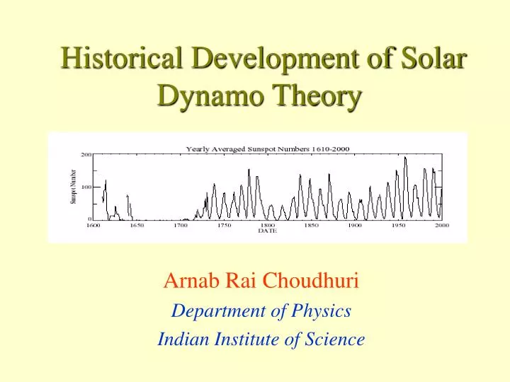
Historical Development of Solar Dynamo Theory Arnab Rai Choudhuri Department of Physics Indian Institute of Science
1844: Schwabe discovered solar cycle1858: Carrington discovered latitudinal drift1904: Maunder invented butterfly diagram
Hale (1908) discovered magnetic fields in sunspotsHale et al. (1919) – Often two large sunspots are seen side by side with opposite polarities A strand of magnetic flux has come through the surface!
Magnetogram map (white +ve, black –ve)Polarity is opposite (i) between hemispheres; (ii) from one 11-yr cycle to next >> 22-yr period Tilt of bipolar regions increases with latitude - Joy’s law (Joy 1919)
Parker (1955) suggested oscillation between the toroidal and poloidal fields. Babcock & Babcock (1955) detected the weak poloidal field (~ 10 G)
The polar fields and the sunspot number as functions of time Polar field data from Wilcox Solar Observatory
Babcock and Babcock (1955) – Weak fields outside sunspots (< 10 G) Unipolar patches shift poleward with solar cycle – Bumba & Howard (1965), Howard & LaBonte (1981), Makarov & Sivaraman (1989), Wang et al. (1989) Hinode found this field to be concentrated in kilogauss patches (Tsuneta et al. 2008)
Polar field reverses at the time of sunspot maximum. Weak, diffuse fields must be another manifestation of solar cycle – ignored by early theorists!
Interaction between velocity & magnetic fields in MHD For compressible fluids, continuity and energy equations also have to be solved. • Two approaches to dynamo theory: • Direct numerical simulation (DNS) • Kinematic model - v assumed given, solve only the induction equation
Early efforts in DNS of solar dynamo by Gilman in 1980s Glatzmaier & Roberts (1996) successfully simulate the geodynamo and find geomagnetic reversals • Challenges for DNS of solar dynanmo • Strong statification (density, pressure) within convection zone • Largest relevant scales (106 km) differ from smallest scales (102 km) by 4 orders
Our theoretical understanding of velocity patterns in the convection zone (differential rotation, meridional circulation) is very limited. Until we can do successful DNS of velocity fields, we have no hope for realistic DNS of the dynamo. Recent DNS are of exploratory nature and have not reached the stage of detailed comparison with observations (Brandenburg, Nordlund, Brun, Miesch, Toomre) Kinematic models use the velocity fields discovered by helioseismology and are able to model many aspects of observational data by assigning suitable values to different parameters
Induction equation: Is it possible to find v and B such that B turns out to be constant in time? Cowling’s anti-dynamo theorem (1934) – axisymmetric solution not possible. Parker’s turbulent dynamo (1955) – toroidal and poloidal fields sustain each other.
Axisymmetric magnetic field Poloidal Component Responsible for weak fields Toroidal Component Gives rise to sunspots Differential rotation – produces toroidal field from poloidal field
Parker’s mechanism of generation of poloidal field from toroidal field – α-effect Parker obtained propagating wave solution
Mean field MHD (Steenbeck, Krause & Radler 1966) Fluctuations around the average Substituting in induction equation and averaging where First order smoothing approximation: where Dynamo equation
Dynamo equation in spherical geometry Mangnetic field with Velocity field On substituting in the dynamo equation T1 T2 T1 >> T2 : αω dynamo (e.g. solar & stellar dynamos) T2 >> T1 : α2 dynamo(e.g. planetary dynamos)
The αω dynamo equation in rectangular geometry can be solved analytically – model for solar cycle? (Parker 1955) Steenbeck & Krause (1969) solved in spherical geometry and obtained the first theoretical butterfly diagram Parker-Yoshimura sign rule (Parker 1955; Yoshimura 1975) for poleward propagation Detailed convection zone dynamo models: Roberts (1972), Kohler (1973), Yoshimura (1975), Stix (1976)
Magnetoconvection Linear theory – Chandrasekhar 1952 Nonlinear evolution – Weiss 1981; . . . Sunspots are magnetic field concentrations with suppressed convection Magnetic field probably exists as flux tubes within the solar convection zone
Tachocline – strong differential rotation, generation of toroidal magnetic field Flux Tube Usually the inside is under-dense Magnetic buoyancy(Parker 1955) Very destabilizing within the convection zone, but much suppressed below its bottom
Difficulties with convection zone dynamos – Magnetic buoyancy will remove magnetic flux from convection zone too quickly (Parker 1975; Moreno-Insertis 1983) Spiegel & Weiss (1980) and van Ballegooijen (1982) proposed that the dynamo operates in the overshoot layer at the base of the convection zone. This was before helioseismology discovered the tacholine!!! Models of interface dynamo – DeLuca & Gilman 1986; Choudhuri 1990; Parker 1993; Charbonneau & MacGregor 1997
3D dynamics of flux tubes in solar convection zone based on Spruit (1981) thin flux tube equation (Choudhuri & Gilman 1987; Choudhuri 1989; D’Silva & Choudhuri 1993; Fan, Fisher & DeLuca 1993; Caligari et al. 1995) Early dynamo models suggested B at bottom to be 10,000 G, but such fields are diverted by Coriolis force (Choudhuri & Gilman 1987) Only 100,000 G fields can emerge at sunspot latitudes
Joy’s Law (1919) – Tilts of bipolar sunspots increase with latitude Figure from D’Silva & Choudhuri (1993) – First quantitative explanation! Only 100 kG = 100,000 G fields match observations!
Alternative mechanism for poloidal field generation (Babcock 1961; Leighton 1969) Decay of tilted bipolar sunspots Toroidal field > bipolar sunspots > poloidal field The original idea of Parker (1955) and Steenbeck, Krause & Radler (1966) involved twisting of toroidal field by helical turbulence – not possible if toroidal field is 100,000 G.
Magnetic fluxes from active regions diffuse and get advected by meridional circulation Dikpati & Choudhuri (1994) – Flux transport in meridional plane with interface dynamo as source Wang, Nash & Sheeley (1989) – Surface flux transport model with actual sunspots as source
The dynamo cycle - A modified version of the original idea due to Parker (1955) Wang, Sheeley & Nash (1991) demonstrated the feasibility of such a dynamo with a 1D model Is the condition satisfied??
Flux transport dynamo in the Sun (Choudhuri, Schussler & Dikpati 1995; Durney 1995) Differential rotation > toroidal field generation Babcock-Leighton process > poloidal field generation Meridional circulation carries toroidal field equatorward & poloidal field poleward
From Choudhuri, Schussler & Dikpati (1995) – Meridional circulation can overcome Parker-Yoshimura sign rule Without meridional circulation With meridional circulation • Important time scales in the dynamo problem • Ttach – Diffusion time scale in the tachocline • Tconv – Diffusion time scale in convection zone • Tcirc – Meridional circulation time scale Ttach > Tcirc > Tconv : Choudhuri, Nandy, Chatterjee, Jiang, Karak, Hotta, Munoz-Jaramillo ... Ttach > Tconv > Tcirc: Dikpati, Charbonneau, Gilman, de Toma…
Basic Equations Magnetic field Velocity field The code Surya solves these equations For a range of parameters, the code relaxes to periodic solutions (Nandy & Choudhuri 2002)
Results from detailed model of Chatterjee, Nandy & Choudhuri (2004) Butterfly diagrams with both sunspot eruptions and weak field at the surface > Reasonable fit between theory & observation
Conclusion • Different phases of solar dynamo models • ~ 1955 – 1980: Convection zone dynamos • ~ 1980 – 1995: Interface dynamo at the tachocline • ~ 1995 – : Flux transport dynamo • Toroidal field generation in tachocline by differential rotation • Poloidal field generation at surface by Babcock-Leighton mechanism • Advection by meridional circulation The solar cycle is probably produced by a flux transport dynamo involving the following processes: