Download
1 / 17
170 likes | 486 Vues
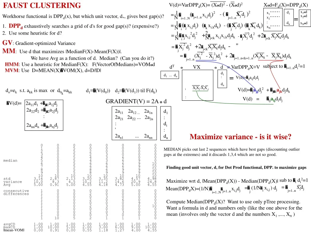
X o d=F d (X)=DPP d (X). d 1. x 1 o d. x 1 x 2 : x N. x 2 o d. =. - ( j=1..n X j d j ) 2. = i=1..N ( j=1..n x i,j d j ) 2. x N o d. d n. V(d) ≡ VarDPP d (X)= (X o d) 2 - (X o d) 2. = i ( j x i,j d j ). - ( j X j d j ). ( k X k d k ).

E N D
Xod=Fd(X)=DPPd(X) d1 x1od x1 x2 : xN x2od = - ( j=1..nXj dj)2 = i=1..N(j=1..nxi,jdj)2 xNod dn V(d)≡VarDPPd(X)= (Xod)2 - (Xod)2 = i(jxi,jdj) - (jXj dj) (kXk dk) (kxi,kdk) + j<kxi,jxi,kdjdk sub to i di2=1 = ijxi,j2dj2 Maximize wrt d, |Mean(DPPd(X)) - Median(DPPd(X)| Mean(DPPdX)=(1/N)i=1..Nj=1..nxi,jdj = j=1..n Xjdj =j (1/Nixi,j ) dj 1 1 1 2 N N N N +2j<kXjXkdjdk - " = jXj2 dj2 +2j<kXjXkdjdk - jXj2dj2 2a11d1 V(d)= +j1a1jdj do=ek s.t. akk is max or d0k=akk d1≡(V(d0)) d2≡(V(d1)) til F(dk) XjXk)djdk ) +(2j=1..n<k=1..n(XjXk- 2a22d2 = j=1..n(Xj2 - Xj2)dj2 + +j2a2jdj : 2anndn +jnanjdj V(d)=jajjdj2 V(d) = ijaijdidj + jkajkdjdk subject to i=1..ndi2=1 dTo VX o d = VarDPPdX≡V d1 : dn V i XiXj-XiX,j : d1 ... dn = V(d)=ijaijdidj MEDIAN picks out last 2 sequences which have best gaps (discounting outlier gaps at the extremes) and it discards 1,3,4 which are not so good. Finding good unit vector, d, for Dot Prod functional, DPP. to maximize gaps GRADIENT(V) = 2A o d 2a11 2a12 ... 2a1n 2a21 2a22 ... 2a2n : ' 2an1 ... 2ann d1 : di : dn Compute Median(DPPd(X)? Want to use only pTree processing. Want a formula in d and numbers only (like the one above for the mean (involves only the vector d and the numbers X1 ,..., Xn ) FAUST CLUSTERING Workhorse functional is DPPd(x), but which unit vector, d*, gives best gap(s)? 1. DPPd exhaustively searches a grid of d's for good gap(s)? (expensive?) 2. Use some heuristic for d? GV: Gradient-optimized Variance MM: Use d that maximizes |MedianF(X)-Mean(F(X))|. We have Avg as a function of d. Median? (Can you do it?) HMM: Use a heuristic for MedianF(X): F(VectorOfMedians)=VOMod MVM: Use D=MEAN(X)VOM(X), d=D/|D| Maximize variance - is it wise? 0 0 0 0 0 0 0 0 1 0 5 0 0 0 0 0 2 0 5 2 0 0 0 0 3 0 5 2 3 0 0 0 4 0 5 4 3 6 0 0 median 5 0 5 4 3 6 9 0 6 0 5 6 6 6 9 10 7 0 5 6 6 6 9 10 8 0 5 8 6 9 9 10 9 0 5 8 9 9 9 10 10 10 10 10 10 10 10 10 std 3.16 2.87 2.13 3.20 3.35 3.82 4.57 4.98 variance 10.0 8.3 4.5 10.2 11.2 14.6 20.9 24.8 Avg 5.00 0.91 5.00 4.55 4.18 4.73 5.00 4.55 consecutive 1 0 5 0 0 0 0 0 differences 1 0 0 2 0 0 0 0 1 0 0 0 3 0 0 0 1 0 0 2 0 6 0 0 1 0 0 0 0 0 9 0 1 0 0 2 3 0 0 10 1 0 0 0 0 0 0 0 1 0 0 2 0 3 0 0 1 0 0 0 3 0 0 0 1 10 5 2 1 1 1 0 avgCD 1.00 1.00 1.00 1.00 1.00 1.00 1.00 1.00 maxCD 1.00 10.00 5.00 2.00 3.00 6.00 9.00 10.00 ||mean-VOM| 0.00 0.91 0.00 0.55 1.18 1.27 4.00 4.55
MVM C11 F-MN gp2 0 1 1 1 1 1 2 3 1 3 3 2 5 2 1 6 1 2 8 2 2 10 2 1 11 1 1 12 4 1 13 1 2 15 2 WINE GV GM ACCURACY WINE GV 62.7 MVM 66.7 GM 81.3 .11 .19 .96 .19 209 -.02 .41 .91 0 232 C1(F-MN) gp3 0 1 1 1 6 1 2 5 1 3 2 1 4 4 1 5 8 1 6 8 1 7 4 1 8 3 1 9 7 1 10 1 1 11 4 1 12 6 1 13 4 1 14 2 1 15 3 1 16 3 1 17 2 1 18 2 1 19 3 1 20 4 1 21 6 1 22 4 1 23 1 1 24 2 1 25 4 1 26 1 1 27 1 2 29 2 1 30 2 2 32 1 3 35 1 1 36 1 1 37 1 1 38 1 1 39 4 1 40 2 2 42 2 2 44 1 1 45 2 2 47 4 1 48 2 1 49 1 1 50 1 3 53 1 1 54 2 1 55 2 [0.12) 1L 0H F-MN Ct gp8 0 1 12 12 1 3 15 2 13 28 1 2 30 1 2 32 2 2 34 1 1 35 2 3 38 1 8 46 1 1 47 3 10 57 1 1 58 1 1 59 1 1 60 1 2 62 1 2 64 1 1 65 1 1 66 1 1 67 4 1 68 2 1 69 1 1 70 1 2 72 3 1 73 1 1 74 3 1 75 2 1 76 1 1 77 1 2 79 1 3 82 1 1 83 1 1 84 2 1 85 1 1 86 1 2 88 2 1 89 4 1 90 2 1 91 1 1 92 6 1 93 3 1 94 5 1 95 4 2 97 5 1 98 2 1 99 1 1 100 4 1 101 7 1 102 4 1 103 2 1 104 3 1 105 6 1 106 3 1 107 8 1 108 10 1 109 2 1 110 4 1 111 5 1 112 2 1 113 4 1 114 1 .07 .15 .98 .12 588 -.01 .26 .97 .00 608 (F-MN) gp8 0 1 1 1 4 1 2 4 1 3 5 1 4 4 1 5 6 1 6 8 1 7 6 1 8 4 1 9 5 1 10 2 1 11 3 1 12 7 1 13 4 1 14 3 1 15 2 1 16 2 1 17 3 1 18 4 1 19 3 1 20 4 1 21 1 1 22 7 1 23 2 1 24 4 1 25 1 1 26 1 1 27 1 1 28 1 1 29 1 1 30 1 1 31 1 1 32 1 3 35 1 2 37 3 1 38 1 1 39 1 1 40 3 1 41 3 3 44 2 1 45 2 1 46 4 1 47 2 2 49 1 2 51 1 1 52 1 3 55 1 1 56 1 1 57 1 9 66 2 1 67 2 8 75 1 4 79 2 1 80 1 2 82 2 1 83 1 2 85 1 13 98 1 2 100 1 3 103 1 11 114 1 -.05 -.31 -.95 -.01 605 .01 -.27 -.96 -.0 608 XF-M gp3 0 1 11 11 1 4 15 1 1 16 1 13 29 1 1 30 1 2 32 2 2 34 1 1 35 2 4 39 1 8 47 2 1 48 2 9 57 1 1 58 1 1 59 1 2 61 1 2 63 1 2 65 1 1 66 1 1 67 1 1 68 5 1 69 2 1 70 1 3 73 3 1 74 3 1 75 1 1 76 2 1 77 2 2 79 1 3 82 1 1 83 1 1 84 1 1 85 1 1 86 1 1 87 1 1 88 1 1 89 1 1 90 4 1 91 2 1 92 7 1 93 1 1 94 5 1 95 4 1 96 2 1 97 3 1 98 2 1 99 2 1 100 3 1 101 4 1 102 7 1 103 3 1 104 2 1 105 6 1 106 3 1 107 5 1 108 9 1 109 6 1 110 4 1 111 5 1 112 4 1 113 4 1 114 1 _4L2H ___ _ [12,28) 1L2H _2L1H 2L 0H C1 -.11 -.02 -.86 .5 43 -.05 -.4 -.92 .01 68 C7F-M*3 g3 0 1 3 3 1 2 5 1 4 9 2 6 15 1 3 18 1 2 20 1 1 21 1 1 22 3 3 25 2 3 28 1 2 30 3 1 31 2 1 32 1 1 33 1 1 34 2 1 35 1 1 36 3 3 39 2 1 40 1 1 41 2 3 44 1 2 46 3 2 48 1 2 50 2 2 52 1 1 53 1 1 54 1 1 55 1 1 56 2 1 57 1 1 58 2 1 59 2 1 60 2 1 61 1 1 62 1 1 63 2 2 65 1 1 66 1 1 67 1 1 68 1 1 69 3 1 70 1 1 71 1 1 72 1 1 73 1 1 74 2 1 75 2 1 76 1 1 77 3 1 78 4 1 79 3 1 80 4 1 81 1 1 82 1 1 83 1 2 85 2 1 86 2 2 88 3 1 89 2 2 91 2 2 93 4 3 96 1 _0L 2H _0L 2H C2 3L5H -.08 .59 -.8 -.07 80 .08 .83 -.56 -.01 95 C5 g3 0 1 4 4 1 8 12 1 3 15 1 2 17 1 2 19 1 4 23 1 1 24 1 2 26 1 1 27 1 2 29 3 2 31 1 1 32 1 1 33 1 ___ _ [28,46) 2L6H 1L1H ___ _ [46,57) 2L2H .05 .59 -.293 .75 18 -.1 .9 -.3 .1 34 C6*8 16 0 1 4 4 2 16 20 1 11 31 1 37 68 1 15 83 1 15 98 1 8 106 1 11 117 1 1 118 2 _2L4H C71 C121 max thin 0 1 1 1 6 1 2 5 1 3 3 1 4 3 1 5 8 1 6 8 1 7 4 1 8 7 1 9 3 1 10 1 1 11 5 1 12 6 1 13 3 1 14 2 1 15 3 1 16 3 1 17 4 _2L5H C3 _0L 1H C4 _3L 0H C1 F-M Ct g3 0 1 1 1 2 1 2 2 3 5 1 1 6 1 1 7 4 1 8 2 2 10 2 1 11 1 2 13 2 1 14 1 1 15 1 1 16 5 2 18 1 2 20 2 3 23 1 1 24 1 1 25 1 1 26 2 2 28 1 1 29 1 1 30 5 1 31 2 1 32 1 1 33 4 1 34 5 1 35 4 1 36 4 1 37 2 1 38 3 1 39 3 1 40 2 1 41 4 1 42 3 1 43 5 1 44 3 1 45 4 1 46 5 1 47 4 1 48 3 1 49 11 1 50 5 1 51 3 1 52 5 1 53 4 1 54 4 1 55 1 _1L2H ___ 4L2H _0L 1H C4 _1L 2H ___ 0L 2H _2L 3L2H 23L 25H 6L 21H _1L6H 5L5H _2L 12H _9L 7H C5 .19 .8 -.54 .18 7 -.21 .7 -.7 -.09 9 C763F-M*8 g8 0 2 16 16 1 13 29 1 12 41 2 4 45 1 7 52 1 4 56 1 7 63 1 8 71 2 _1L4H .01 -.27 -.96 -.01 23 -.04 -.43 -.9 .03 24 C76*4 g3 0 1 31 31 1 3 34 1 1 35 2 2 37 1 2 39 2 2 41 1 2 43 1 1 44 1 2 46 3 3 49 1 1 50 1 1 51 2 1 52 1 1 53 2 2 55 2 2 57 2 3 60 1 2 62 2 1 63 1 2 65 3 1 66 2 3 69 1 1 70 1 1 71 2 2 73 2 1 74 1 1 75 2 1 76 3 1 77 2 1 78 2 1 79 3 1 80 3 2 82 1 2 84 1 2 86 2 1 87 1 1 88 1 2 90 2 1 91 2 3 94 2 2 96 2 1 97 2 C11 10L 13H C12 0L 2H ___ _1L 0H ___ _0L 1H _2L 0H [0.35) C11 38L68H C12 F-M gp2 0 1 1 1 8 1 2 3 1 3 2 1 4 4 1 5 11 1 6 8 1 7 2 1 8 6 1 9 4 1 10 3 1 11 4 1 12 4 1 13 5 1 14 3 1 15 3 1 16 4 2 18 2 1 19 5 1 20 6 1 21 4 1 22 1 1 23 2 1 24 3 1 25 3 3 28 2 1 29 2 2 31 1 4L 8H C6 _2L4H 4L8H C763 _0L 2H -.21 .34 -.91 .9 8 C766 *16 g4 0 1 30 30 1 2 32 1 7 39 1 1 40 1 1 41 1 1 42 1 4 46 1 2 48 1 2 50 2 5 55 1 3 58 1 7 65 1 2 67 1 5 72 1 3 75 2 2 77 1 1 78 4 2 80 1 3 83 1 1 84 2 4 88 1 1 89 1 11 100 1 4 104 1 11 115 1 _0L 1H [35,53) C12 10L13H ___ _ 2L9H _2L 0H ___ [53,56) 3L 2H _3L 1H 29L 46H ___ _ 1L8H 51L 83H [0.66) C1 _1L 3H ___ _ [66,75) 2L2H _2L 0H _2L 0H 7L 19H 2L2H ___ _ [75,98) 2L6H 0L 1H ___ [57,115) 51L 83H C1 _4L 8H ___ _ [98,115) 2L2H 17L 15H C766 _2L 0H 38L 68H C7 _0L 2H ___ 28L 44H C76 1L _1L 0H ___ _ 3L3H
SEEDS GV MVM 256 36 10 32 akk .98 .14 .04 .12 0 .00 -.00 .96 .29 3 C6 10(F-M) g12 0 3 10 10 1 12 22 3 10 32 3 9 41 2 7 48 1 ACCURACY SEEDS WINE GV 94 62.7 MVM 93.3 66.7 GM 96 81.3 219 31 14 29 akk d1 d2 d3 d4 V(d .98 .14 .06 .13 9 .98 .14 .06 .13 9 10(F-MN) gp6 0 2 1 1 10 1 2 5 1 3 1 6 9 3 1 10 10 1 11 10 1 12 2 6 18 2 1 19 3 1 20 7 1 21 2 1 22 1 1 23 3 6 29 6 1 30 4 1 31 7 1 32 1 6 38 1 1 39 2 1 40 6 1 41 5 1 42 1 7 49 3 1 50 1 2 52 7 1 53 2 7 60 1 2 62 4 1 63 3 8 71 5 1 72 2 2 74 1 6 80 5 1 81 8 1 82 5 1 83 3 9 92 2 10 102 1 1 103 2 1 104 1 10(F-MN)gp6 0 2 1 1 10 1 2 5 1 3 1 6 9 3 1 10 10 1 11 10 1 12 2 6 18 2 1 19 3 1 20 7 1 21 2 1 22 1 1 23 3 6 29 6 1 30 4 1 31 7 1 32 1 6 38 1 1 39 2 1 40 6 1 41 5 1 42 1 7 49 3 1 50 1 2 52 7 1 53 2 7 60 1 2 62 4 1 63 3 8 71 5 1 72 2 2 74 1 6 80 5 1 81 8 1 82 5 1 83 3 9 92 2 10 102 1 1 103 2 1 104 1 ___ ___ [0,9) 0k 0r 18c C1 ___ ___ [0,9) 0k 0r 18c C1 ___ ___ [9,18) 1k 0r 24c C2 GM ___ ___ [9,18) 1k 0r 24c C2 .794 -.403 -.304 .337 6 0.957 .156 -.205 .132 9 10(F-MN) gp3 0 1 2 2 1 2 4 4 2 6 3 2 8 7 2 10 2 2 12 1 2 14 1 2 16 10 2 18 10 1 19 2 3 22 2 1 23 2 1 24 1 1 25 1 2 27 4 2 29 4 2 31 4 2 33 2 5 38 3 1 39 3 2 41 7 2 43 2 2 45 2 1 46 1 2 48 1 1 49 1 1 50 4 2 52 5 1 53 1 1 54 3 3 57 2 2 59 3 2 61 3 1 62 1 2 64 3 2 66 3 3 69 5 7 76 1 2 78 2 2 80 2 2 82 4 2 84 1 2 86 1 2 88 4 1 89 1 1 90 8 2 92 5 11 103 2 1 104 1 1 105 1 1 106 1 2 108 1 ___ ___ [18,29) 10k 0r 8c C3 ___ ___ [18,29) 10k 0r 8c C3 ___ ___ [29,38) 18k 0r 0c C4 ___ ___ [29,38) 18k 0r 0c C4 ___ ___ [38,49) 13k2r 0c C5 -.577 .577 .577 .000 1 .119 .112 .986 .000 3 C2: 10(F-MN) gp10 0 1 10 10 2 1 11 3 10 21 3 10 31 5 10 41 1 10 51 1 11 62 1 1 63 1 ___ ___ [0,22) 0k 0r 42c C1 ___ ___ [38,49) 13k2r 0c C5 ___ ___ [49,60) 7k 6r 0c C6 ___ ___ [0,31) 9k 0r 0c C21 ___ ___ [49,60) 7k 6r 0c C6 ___ ___ [60,71) 1k 7r 0c C7 ___ ___ [31,41) 1k 0r 4c C22 ___ ___ [60,71) 1k 7r 0c C7 ___ ___ [71,80) 0k 8r 0c C8 ___ ___ [22,33) 10k 0r 8c C2 ___ ___ [41,64) 0k 0r 4c C23 ___ ___ [71,80) 0k 8r 0c C8 ___ ___ [80,92) 0k 21r 0c C9 ___ ___ [92,102) 0k 2r 0c Ca ___ ___ [80,92) 0k 21r 0c C9 ___ ___ [92,102) 0k 2r 0c Ca ___ ___ [102,105) 0k 4r 0c Cb C3 200(F-MN)gp12 0 2 12 12 3 12 24 3 12 36 5 12 48 1 12 60 1 12 72 1 40 112 2 ___ ___ [102,105) 0k 4r 0c Cb ___ ___ [33,57) 33k2r 0c C3 C3 .97 .15 .09 .14 0 0 .07 1 0 4 10F-M g9 0 2 10 10 3 10 20 3 10 30 4 1 31 1 9 40 1 10 50 1 11 61 1 9 70 2 ___ ___ [0,35) 8k 0r 0c ___ ___ [0,10) 2k 0r 0c ___ ___ [35,48) 2k 0r 3c ___ ___ [10,20) 2k 0r 1c -.832 -.282 .134 -.458 0 -.44 .00 -.87 -.22 2 C4: 10(F-MN) gp21 0 3 11 11 2 20 31 3 21 52 3 27 79 1 20 99 3 ___ ___ [20,30) 2k 0r 1c ___ ___ [48,72) 0k 0r 2c ___ ___ [57,69) 6k 9r 0c C4 ___ ___ [69,76) 1k4r 0c C6 ___ ___ [30,40) 4k 0r 1c ___ ___ [72,113) 0k 0r 3c ___ ___ [40,50) 0k 0r 1c ___ ___ [50,61) 0k 0r 1c ___ ___ [61,70) 0k 0r 1c ___ ___ [0,52) 1k7r C41 ___ ___ [70,71) 0k 0r 2c ___ ___ [52,79) 1k2r C42 C6 200(F-MN)gp12 0 3 12 12 1 38 50 3 10 60 1 2 62 3 12 74 2 ___ ___ [79100) 4k 0r C43 ___ ___ [0,50) 4k 0r 0c ___ ___ [50,60) 1k 0r 2c ___ ___ [76,103) 0k 26r 0c C7 ___ ___ [0,22) 4k 0r 0c ___ ___ [60,74) 1k 0r 3c ___ ___ [74,75) 1k 0r 1c ___ ___ [103,109) 0k 6r 0c C8 ___ ___ [22,49) 3k 6r 0c
ACCURACY CONCRETE IRIS SEEDS WINE GV 76 82.7 94 62.7 MVM 78.8 94 93.3 66.7 GM 94.7 96 81.3 MVM C2 3762 808 2260 266 d1 d2 d3 d4 .84 .18 .51 .06 64 .57 .22 .71 .34 82 .51 .22 .74 .38 83 (F-MN)*3 Ct gp3 0 1 2 2 1 1 3 1 2 5 1 15 20 2 3 23 1 3 26 2 2 28 1 1 29 1 2 31 1 2 33 2 2 35 2 2 37 1 1 38 3 1 39 1 1 40 1 1 41 1 1 42 1 4 46 1 1 47 2 2 49 1 1 50 1 1 51 1 2 53 1 1 54 2 2 56 1 2 58 1 1 59 2 2 61 2 1 62 2 1 63 3 1 64 1 1 65 2 2 67 3 1 68 2 1 69 1 1 70 2 1 71 2 1 72 2 2 74 1 1 75 1 2 77 1 1 78 1 1 79 1 2 81 1 2 83 1 1 84 1 3 87 2 1 88 1 1 89 1 1 90 2 1 91 1 1 92 2 3 95 1 1 96 2 1 97 1 2 99 1 2 101 2 2 103 1 3 106 3 3 109 1 1 110 1 1 111 1 .81 .28 -.28 .42 13... .53 .23 .73 .37 39 C12 4*F-M g3 0 2 4 4 1 4 8 2 2 10 1 2 12 1 2 14 1 3 17 1 1 18 1 2 20 1 1 21 1 1 22 1 2 24 3 1 25 1 2 27 1 1 28 1 2 30 1 4 34 1 2 36 2 2 38 1 3 41 2 3 44 1 2 46 2 2 48 1 2 50 1 2 52 2 2 54 1 1 55 1 1 56 1 1 57 1 1 58 3 1 59 1 1 60 2 2 62 1 1 63 4 2 65 1 1 66 1 1 67 1 1 68 1 1 69 3 3 72 1 2 74 1 2 76 1 2 78 1 1 79 1 3 82 1 2 84 1 1 85 1 4 89 1 1 90 1 2 92 1 1 93 1 IRIS GM GV ACCURACY IRIS SEEDS WINE GV 82.7 94 62.7 MVM 94 93.3 66.7 GM 94.7 96 81.3 C23 F-M*3 g3 3847 818 2284 257 .96 .22 .06 -.14 15 0 1 6 6 1 2 8 1 4 12 1 3 15 1 1 16 1 2 18 2 8 26 1 2 28 1 1 29 1 1 30 1 2 32 1 1 33 1 3 36 1 3 39 2 1 40 1 1 41 2 1 42 2 2 44 2 2 46 1 1 47 2 5 52 1 1 53 1 3 56 1 1 57 1 3 60 1 1 61 1 1 62 1 2 64 1 6 70 2 5 75 1 2 77 2 3 80 1 9 89 1 8 97 1 F-MN gp8 0 2 3 3 5 1 4 5 1 5 14 1 6 11 1 7 6 1 8 1 1 9 5 1 10 1 5 15 1 8 23 1 2 25 2 2 27 1 2 29 1 1.. 68 1 .88 .09 -.98 -.18 168 -.29 .13 -.88 -.36 417 -.36 .09 -.86 -.36 420 F-MN Ct gp5 0 1 3 3 2 1 4 1 2 6 1 1 7 1 2 9 2 1 10 1 2 12 3 1 13 1 1 14 3 1 15 4 1 16 2 1 17 3 1 18 1 1 19 6 1 20 3 1 21 1 1 22 2 1 23 2 1 24 6 1 25 7 1 26 2 1 27 3 1 28 2 1 29 6 1 30 3 1 31 2 1 32 3 1 33 3 1 34 3 1 35 3 1 36 5 1 37 1 1 38 2 1 39 1 1 40 2 1 41 1 2 43 1 2 45 1 1 46 1 1 47 1 5 52 1 8 60 2 1 61 3 1 62 4 1 63 3 1 64 13 1 65 12 1 66 4 1 67 5 1 68 2 2 70 2 .90 .24 .37 .04 180 .41 -.04 .84 .35 418 .36 -.08 .86 .36 420 F-MN Ct gp3 0 2 2 2 2 1 3 2 1 4 5 1 5 7 1 6 16 1 7 6 1 8 4 1 9 4 1 10 2 8 18 1 5 23 1 2 25 2 2 27 1 2 29 1 1 30 1 1 31 1 1 32 2 1 33 1 1 34 3 1 35 5 1 36 4 1 37 3 1 38 1 1 39 4 1 40 3 1 41 3 1 42 4 1 43 4 1 44 2 1 45 5 1 46 7 1 47 3 1 48 2 1 49 1 1 50 3 1 51 4 1 52 3 1 53 2 1 54 3 1 55 3 1 56 3 1 57 1 1 58 4 3 61 2 1 62 1 1 63 1 2 65 1 1 66 1 1 67 2 3 70 1 ___ 1e 0i -.36 .09 -.86 -.36 105 -.54 -0.17 -.76 -.33 118 C1 2*(F-M g3 0 2 4 4 1 1 5 1 1 6 1 5 11 1 2 13 1 3 16 1 2 18 1 3 21 1 1 22 1 1 23 1 2 25 2 1 26 2 2 28 2 1 29 1 2 31 3 1 32 1 2 34 1 1 35 2 1 36 2 1 37 4 3 40 2 1 41 1 2 43 3 2 45 1 2 47 4 1 48 1 1 49 2 1 50 4 1 51 3 2 53 5 1 54 2 1 55 2 1 56 1 1 57 3 2 59 3 2 61 2 2 63 1 1 64 1 1 65 2 2 67 1 1 68 1 1 69 2 1 70 2 1 71 3 1 72 1 1 73 2 2 75 1 1 76 1 1 77 1 1 78 1 1 79 1 1 80 1 2 82 2 10 92 1 2 94 2 2 96 1 __2e 5i 50s1i C1 C2 ___ 4e 1i C21 ___ 19e1i C22 4(F-) g4 0 1 6 6 1 4 10 1 2 12 1 4 ... 33 2 1 34 1 4 38 1 1 39 1 3 ... 79 1 2 81 1 5 86 1 2 88 2 2 90 1 1 91 1 1 92 2 2 94 1 1 95 1 2 97 1 1 98 1 3 101 2 1 102 2 4 106 1 1 107 1 2 109 1 1 110 2 1 111 2 6 117 1 1 118 1 1 119 1 1 120 1 ___50s1i C1 ___ 6e 0i ___ 18e C221 29e 14i ___ ___ ___ 19e1i C22 ___28i C11 ___ 16e11i 18e 11i C123 ___ 6e ___ 2e ___ 3e2i C221 8F- g5 0 1 7 7 1 4 11 1 5 16 1 1 17 1 3 20 1 1 21 1 2 23 1 1 24 1 5 29 1 3 32 2 2 34 1 1 35 1 4 39 3 5 44 1 3 47 2 3 50 1 3 53 1 4 57 1 3 60 1 3 63 1 1 64 2 5 69 2 1 70 1 3 73 1 1 74 1 1 75 1 4 79 1 1 80 2 2 82 2 1 83 1 1 84 1 2 86 1 4 90 1 5 95 1 ___1e ___ 0e 3i ___ 2e ___ 26i ___ 0e 4i C221 8F-)g5 0 1 7 7 1 4 11 1 5 16 1 1 17 1 3 20 1 1 21 1 2 23 1 1 24 1 5 29 1 3 32 2 2 34 1 1 35 1 4 39 3 5 44 1 3 47 2 3 50 1 3 53 1 4 57 1 3 60 1 3 63 1 1 64 2 5 69 2 1 70 1 3 73 1 1 74 1 1 75 1 4 79 1 1 80 2 2 82 2 1 83 1 1 84 1 2 86 1 4 90 1 5 95 1 ___50e 49i C1 __ 4e1i ___ 3e . -.034 .37 -.31 .87 4 C123 12*F-M g4 0 1 6 6 1 10 16 1 2 18 1 3 21 1 1 22 1 1 23 1 6 29 1 3 32 1 3 35 1 5 40 2 5 45 1 4 49 1 1 50 2 4 54 1 2 56 1 5 61 2 1 62 1 2 64 1 1 65 1 2 67 1 3 70 1 1 71 1 12 83 1 1 84 1 1 85 1 __ 1i . ___ 50e 40i C2 9i C3 ___ 1e . _46e 21i C12 ___9e ___ 5e 1i ___ 4e C13 ___ 27e 16i C23 ___9e . ___ 50s1i C2 ___ 9e1i . __9e2i C2 2(F-)g4 0 1 4 4 1 1 5 1 4 9 1 3 ... 69 1 4 73 1 1 74 1 2 76 2 4 80 1 4 84 1 2 86 2 5 91 1 ___ 9i C24 _ 4e . __9e2i ___ 3e __ 0e 2i . 47e 40i C22 ___ 8i ___ 3i ___ 2e6i . ___ 5e10i ___ _3i ___ 1i ___ 0e 11i ___ 2e1i ___ 5e11i
CONCRETE GM C11 F-/4 g4 0 4 2 2 1 2 4 4 2 6 25 2 8 2 1 9 7 1 10 4 1 11 9 2 13 3 1 14 6 1 15 4 1 16 1 3 19 5 4 23 2 3 26 5 1 27 4 1 28 9 1 29 5 2 31 6 1 32 5 3 35 6 5 40 2 C232 g2 F-M/8 0 1 1 1 1 1 2 2 1 3 1 2 5 2 1 6 1 1 7 2 1 8 2 1 9 1 7 16 1 1 17 3 1 18 2 2 20 7 1 21 8 1 22 7 1 23 1 2 25 2 1 26 3 1 27 2 1 28 3 1 29 1 1 30 1 1 31 2 2 33 1 1 34 4 1 35 3 3 38 3 1 39 8 11 50 2 1 51 1 MVM (F-)/4 gp4 C23 g3 F-M/8 0 2 2 2 1 1 3 3 1 4 3 1 5 1 1 6 1 1 7 6 1 8 1 1 9 8 1 10 2 1 11 6 1 12 2 1 13 5 1 14 2 1 15 2 3 18 1 1 19 7 1 20 1 1 21 3 1 22 1 1 23 2 1 24 4 1 25 1 2 27 8 1 28 9 1 29 4 2 31 2 1 32 1 1 33 3 1 34 3 2 36 7 1 37 12 2 39 1 1 40 1 1 41 1 1 42 6 6 48 1 2 50 2 0L 32M 13H 11L 13M 54H ACCURACY CONCRETE IRIS SEEDS WINE GV 76 82.7 94 62.7 MVM 78.8 94 93.3 66.7 GM 83 94.7 96 81.3 C2-.6 .2 -.07 .771 6882.. -.72 .19 -.40 .54 9251 .38 .14 -.79 .46 11781 GV F-m/8 g4 C2 0 1 2 2 1 1 3 1 2 5 2 3 8 1 2 10 1 1 11 1 5 16 1 2 18 1 5 23 1 1 24 1 1 25 2 1 26 2 1 27 1 2 29 4 1 30 2 1 31 2 1 32 1 1 33 3 2 ... 1s 65 1 X g4 (F-MN)/8 0 2 2 2 1 2 4 2 1 5 1 3 8 2 3 11 1 1 12 3 2 14 4 1 15 3 1 16 3 1 17 2 1 18 3 1 19 6 1 20 3 1 21 3 1 22 2 1 23 5 1 24 4 1 25 3 1 26 6 1 27 3 1 28 1 1 29 6 1 30 3 1 31 2 1 32 3 1 33 3 1 34 1 2 36 3 1 37 1 1 38 2 1 39 3 1 40 5 1 41 1 1 42 6 1 43 1 1 44 3 2 46 5 1 47 1 1 48 3 1 49 1 1 50 2 1 51 1 1 52 1 1 53 1 1 54 1 1 55 1 1 56 3 1 57 3 2 59 1 2 61 1 1 62 3 3 65 2 9 74 1 4 78 1 3 81 1 2 83 1 3 86 1 2 88 1 2 90 1 1 91 1 4 95 1 2 97 1 1 98 1 2 100 1 4 104 1 3 107 1 0 1 1 1 1 4 5 1 1 ... 1s 46 4 3 49 1 7 56 1 2 58 1 3 61 1 4 65 1 1 66 1 3 69 1 2 71 1 6 77 1 3 80 1 3 83 1 3 86 1 14 100 1 3 103 1 2 105 1 3 108 2 4 112 1 ___ 2M C2 gp8 (F-MN)/5 0 2 2 2 1 2 4 2 1 5 1 3 8 2 3 11 1 1 12 2 2 14 4 1 15 3 1 16 3 1 17 2 1 18 3 1 19 6 1 20 3 1 21 3 1 22 1 1 23 5 1 24 3 1 25 3 1 26 6 1 27 3 1 28 1 1 29 6 1 30 3 1 31 2 1 32 1 1 33 3 1 34 1 2 36 3 2 38 2 1 39 2 1 40 5 1 41 1 1 42 6 1 43 1 1 44 3 2 46 5 1 47 1 1 48 1 1 49 1 1 50 2 1 51 1 1 52 1 1 53 1 1 54 1 1 55 1 1 56 3 1 57 2 2 59 1 2 61 1 1 62 3 3 65 2 9 74 1 4 78 1 8 86 1 2 88 1 2 90 1 5 95 1 2 97 1 1 98 1 2 100 1 4 104 1 C21 0L 8M 0H C1 43L 33M 55H C22 2M 0H C23 C211 g5 F-M)/4 0 1 6 6 2 1 7 2 5 12 1 1 13 4 1 14 1 1 15 4 2 17 1 1 18 2 1 19 2 2 21 2 1 22 3 1 23 1 1 24 3 4 28 1 14 42 1 2 44 1 1 45 1 3 48 2 2 50 1 5 55 1 2 57 1 1 58 1 5 63 1 1 64 1 7 71 1 11 82 1 16 98 2 g4 F-MN/8 0 1 2 2 1 2 4 1 2 6 1 1 7 1 1 8 1 2 10 1 1 11 1 1 12 1 1 13 1 3 16 2 3 19 1 2 21 1 5 26 1 1 27 1 1 28 2 1 29 2 1 30 1 2 32 5 1 33 2 1 34 2 1 35 1 1 36 3 1 37 3 1 38 3 1 39 5 1 40 3 1 41 7 1 42 6 1 43 3 1 44 5 1 45 1 1 46 3 1 47 3 1 48 4 1 49 7 1 50 4 1 51 6 1 52 10 1 53 3 1 54 4 1 55 8 1 56 5 1 57 3 1 58 7 1 59 2 1 60 2 1 61 1 1 62 2 2 64 1 1 65 2 1 66 1 1 67 2 C21 g4 F-M/4 0 1 1 1 1 3 4 1 3 7 2 1 8 2 1 9 1 2 11 1 2 13 4 1 14 2 1 15 4 1 16 1 2 18 2 1 19 3 1 20 1 1 21 2 1 22 6 2 24 2 1 25 3 1 26 1 2 28 2 2 30 1 1 31 1 2 33 1 4 37 1 1 38 2 1 39 2 1 40 1 1 41 1 1 42 1 1 43 2 1 44 1 1 45 2 1 46 1 1 47 1 1 48 1 1 49 2 2 51 2 4 55 1 1 56 8 1 57 4 1 58 4 1 59 2 1 60 1 1 61 1 2 63 5 2 65 1 2 67 2 1 68 1 3 71 1 1 72 4 1 73 8 1 74 5 1 75 1 8 83 3 1 84 3 1 85 2 1 86 1 99 3 ___5L . C111 3L 23M 49H ___ 7M C2 ___ 4M C3 ___6M C4 ___ 30L 1M 4H C231 g4 F-M/8 0 1 7 ... 1s 12 1 2 14 6 1 15 7 4 19 1 1 20 3 1 21 3 1 22 2 1 23 1 2 25 1 2 27 1 2 29 1 1 30 1 1 31 1 2 33 1 6 39 1 3 42 1 4 46 1 10 56 2 __20L5M . C1F-/4 g4 ___14M 0H C1 C2 0 1 1 1 1 7 8 1 4 12 1 4 16 1 2 18 1 2 20 2 1 21 2 2 ... 1s+2s 71 2 2 73 1 1 74 1 2 76 2 2 78 2 4 82 2 2 84 1 6 90 2 8 98 1 9 107 1 16 123 1 ___ 5L1M . ___ 4M . ___ 2L1M . C211 32L 13M 0H ___5L1M C11 43L 23M 53H _30L8H_ . 3L2M C212 g5 F-M/3 0 1 20 20 1 8 28 1 1 29 2 9 38 1 11 49 1 5 54 1 11 65 1 10 75 2 3 78 1 11 89 1 7 96 1 2 98 1 2 100 1 11 111 2 1 112 1 ___6M2H C212 7L 3M 10H 2L2M1H __6L3M . __1L2H C111 F-/4 g4 0 1 16 16 3 1 17 2 1 18 9 1 19 3 2 21 5 6 27 3 1 28 5 1 29 14 1 30 1 8 38 2 2 40 15 1 41 3 4 45 3 2 47 2 19 66 3 21 87 1 ___1L4M3H ___ __1L ___1L 1M4H ___ 8H 43L 38M 55H C2 0L 14M 0H C1 ___ 3L 2M18H 1L 21M 43L 28M 55H C21 __ 1L 2M 20H C213 4L 7M 38H ___4L 2M8H ___ 8H C214 0L 5M 7H ___ 2M9H ___ ___ . 1H 2M 0L 10M 0H C22 ___ __ 31H ___1L2H
KOSblogs d=UnitSTDVec g>6*avg GV on 22 highest STD KOS wds d=(.46 .16 .03 .32 .71 .07 .06 .03 .09 .03 .10 .10 .19 .04 .16 .14 .01 .02 .04 .02 .00 .02) d=e841 (highest STD). gp=1 Ct=8 C16 . outliers. Some of them are substantial MVM gaps>6*avg DOC W=841 1716 0 ... ... 1379 C0 2427 0 AVG->2.987 0.008 12 kos DPPd gap 24 2682 0 2749 7.574 0.038 0 3029 2983 8.436 0.079 0 42 3402 8.629 0.052 0 2 864 9.184 0.053 0 10 2293 9.462 0.106 1 4 2994 13.45 0.055 0 316 1445 13.66 0.029 0 4 3399 14.05 0.099 0 6 185 14.21 0.156 1 1 2731 14.35 0.143 1 1 2948 14.65 0.066 0 5 1495 14.99 0.014 0 2 804 15.20 0.205 1 1 3177 15.42 0.034 0 6 1316 15.61 0.024 0 2 1335 16.01 0.028 0 3 1637 16.35 0.330 1 1 880 16.86 0.039 0 3 1509 17.03 0.176 1 1 2885 17.21 0.177 1 1 446 18.07 0.863 1 1 1197 18.65 0.005 0 4 3189 19.30 0.644 1 1 1252 20.65 1.352 1 1 2750 13 54 13 2293 13 183 13 2870 13 1222 13 3217 13 1519 13 8 C13 1027 1 ... ... 3427 1 743 C1 2164 14 otlrs 1656 14 3244 14 1709 14 185 15 otlrs 401 15 414 15 893 15 2731 16 otlrs 1396 16 3220 16 3190 16 1832 17 otlr 2852 18 otlrs 3201 18 1234 18 3189 19 otlr 1524 22 otlr 1529 24 otlr 1197 25 otlr 201 27 otlr 1150 29 otlr 1335 34 otlr 1 2 ... ... 2519 2 470 C2 868 3 ... ... 3224 3 274 C3 1882 4 ... ... 3257 4 175 C4 1434 5 ... ... 910 5 127 C5 Cluster size: d=USTDMN-VM 10 7 11 8 15 8 16 9 17 11 21 11 27 12 42 30 48 45 68 87 422 502 2667 2613 GRAVAR 3 3 4 4 4 5 6 6 10 42 316 3029 2753 6 ... ... 549 6 75 C6 1186 7 ... ... 1015 7 79 C7 503 8 ... ... 3156 8 43 C8 2971 9 ... ... 2182 9 39 C9 2868 10 ... ... 1316 10 32 C10 2648 11 ... ... 336 11 18 C11 2983 12 ... ... 3177 12 14 C12 3364 1804 185.38 0.56 0 3365 3399 186.38 1.00 1 3366 980 186.68 0.30 0 3367 1518 187.84 1.15 1 3368 2090 188.45 0.61 1 3369 890 189.10 0.65 1 3370 24 189.74 0.65 1 3371 2435 189.77 0.03 0 3372 804 190.14 0.36 0 3373 930 190.24 0.11 0 3374 1096 191.30 1.06 1 3375 1441 191.39 0.09 0 3376 2885 191.86 0.47 0 3377 2315 191.91 0.05 0 3378 699 192.04 0.13 0 3379 2108 194.34 2.30 1 3380 1316 195.58 1.24 1 3381 991 195.85 0.27 0 3382 1564 196.05 0.20 0 3383 2800 196.37 0.32 0 3384 880 196.62 0.25 0 3385 2038 196.75 0.13 0 3386 481 197.09 0.34 0 3387 480 197.85 0.76 1 3388 295 198.38 0.53 0 3389 1234 200.42 2.04 1 3390 2140 201.46 1.04 1 3391 3353 202.36 0.90 1 3392 3402 202.64 0.28 0 3393 45 202.86 0.21 0 3394 3017 204.63 1.77 1 3395 3365 207.54 2.91 1 3396 2436 207.77 0.24 0 3397 553 209.73 1.96 1 3398 2545 210.52 0.79 1 3399 54 213.63 3.11 1 3400 1933 214.58 0.95 1 3401 3201 216.16 1.57 1 3402 2895 217.18 1.02 1 3403 446 217.83 0.65 1 3404 2302 218.43 0.61 1 3405 2873 219.47 1.04 1 3406 3388 223.00 3.52 1 3407 1509 225.98 2.99 1 3408 32 229.46 3.48 1 3409 3189 231.30 1.84 1 3410 3228 231.43 0.13 0 3411 2107 232.39 0.96 1 3412 1150 232.79 0.40 0 3413 2279 236.69 3.90 1 3414 2289 237.43 0.74 1 3415 2385 238.03 0.60 0 3416 1037 245.93 7.90 1 3417 201 246.72 0.79 1 3418 1252 249.23 2.51 1 3419 1739 250.34 1.11 1 3420 2446 257.59 7.26 1 3421 1637 258.64 1.05 1 3422 3220 260.55 1.91 1 3423 1304 262.67 2.12 1 3424 2355 271.20 8.53 1 3425 232 293.86 22.66 1 3426 3411 299.23 5.37 1 3427 1955 303.42 4.19 1 3428 1832 328.03 24.61 1 3429 1197 335.83 7.81 1 3430 2852 364.01 28.18 1 AvgGp.0085 gp>6*avg ROW KOS F GAP CT 1 1791 0.2270 --- -- 2 1317 0.2920 0.065 1 2668 1602 6.6576 0.007 2667 3090 1390 9.8504 0.004 422 3132 1546 10.278 0.012 42 3148 2662 10.507 0.021 16 3216 505 11.289 0.019 68 3264 2219 11.994 0.027 48 3291 231 12.445 0.039 27 3302 710 12.631 0.038 11 3317 220 12.934 0.023 15 3338 405 13.315 0.028 21 3355 194 13.693 0.009 17 3368 12 14.151 0.078 8 3378 2731 14.590 0.011 10 3392 1096 15.459 0.022 5 avg 63.3 0.1 64 #gaps max 364.0 28.2 0.60 GapThreshold 1 1791 5.67 gap 0 ... ... ... ... ... 8 3389 7.00 0.19 0 9 2397 7.65 0.65 1 10 2841 7.82 0.17 0 ... ... ... ... ... 2621 2334 89.40 0.06 0 2622 1122 90.00 0.60 1 2623 245 90.06 0.06 0 ... ... ... ... ... 3123 3169 132.06 0.00 0 3124 321 132.81 0.75 1 3125 2047 133.05 0.24 0 ... ... ... ... ... 3210 343 145.29 0.37 0 3211 2475 145.89 0.60 1 3212 458 146.10 0.21 0 ... ... ... ... ... 3240 542 151.15 0.09 0 3241 2569 151.76 0.61 1 3242 1143 151.92 0.15 0 ... ... ... ... ... 3285 1803 157.97 0.00 0 3286 2257 158.70 0.73 1 3287 2723 158.77 0.07 0 ... ... ... ... ... 3293 129 159.56 0.32 0 3294 2541 160.45 0.89 1 3295 2870 160.48 0.03 0 ... ... ... ... ... 3301 401 161.38 0.04 0 3302 2918 162.03 0.65 1 3303 100 162.07 0.04 0 ... ... ... ... ... 3312 1157 164.54 0.08 0 3313 185 165.26 0.72 1 3314 685 165.91 0.65 1 3315 2948 166.25 0.34 0 ... ... ... ... ... 3325 190 168.59 0.37 0 3326 2498 169.20 0.61 1 3327 264 169.31 0.11 0 3328 1611 169.64 0.33 0 3329 3052 169.96 0.32 0 3330 1002 170.43 0.47 0 3331 1628 170.64 0.20 0 3332 1241 171.80 1.16 1 3333 3155 172.00 0.20 0 ... ... ... ... ... 3342 861 173.84 0.15 0 3343 2509 174.98 1.13 1 3344 2293 175.65 0.67 1 3345 1257 175.67 0.02 0 3346 2776 176.04 0.37 0 3347 1422 177.15 1.11 1 3348 12 177.24 0.09 0 3349 183 177.26 0.02 0 3350 620 177.29 0.03 0 3351 679 179.08 1.79 1 3352 462 179.15 0.07 0 3353 3404 180.02 0.88 1 3354 1850 180.79 0.76 1 3355 3342 181.21 0.43 0 3356 1396 183.04 1.82 1 3357 2982 183.26 0.22 0 ___ ___ gap=.65 Ct=9 C1 ___ ___ gap=.6 Ct=2613 C2 ___ ___ gap=.75 Ct= 502 C3 ___ ___ gap=.6 Ct= 87 C4 ___ ___ gap=.61 Ct=30 C5 ___ ___ gap=.73 Ct=45 C6 ___ ___ gap=.89 Ct=8 C7 ___ ___ gap=.65 Ct=8 C8 ___ ___ gp=.72 Ct= 11 C9 ___ ___ gp=.65 Ct=1 outlr ___ ___ gp=.61 Ct=12 C11 ___ ___ gp=1.2 Ct=6 C12 ___ ___ gp=1.1 Ct=11 C13 ___ ___ gap=.67 Ct=1 utlr ___ ___ gp=1.1 Ct=3 C15 ___ ___ gp=1.8 Ct=4 C16 ___ ___ gp=1.8 Ct=5 otl;r
FAUST Clustering using Fpq(x)=RND[(x-p)o(q-p)/|q-p|-minF] onSpaeth image (p=avg 0 0 0 0 0 0 0 0 1 0 0 0 0 0 0 0 1 0 0 0 0 0 0 0 0 1 0 0 0 0 0 0 0 1 0 0 0 0 0 0 0 1 0 0 0 0 0 0 0 1 0 0 0 0 0 1 0 0 0 0 0 0 0 0 0 1 0 0 0 0 0 0 1 0 0 0 0 0 0 0 0 0 0 1 0 0 0 0 0 0 0 0 1 0 0 0 0 0 0 0 1 0 0 0 0 0 0 0 0 0 1 0 0 0 0 0 0 1 0 0 0 0 0 0 0 0 0 0 0 1 0 0 0 0 0Level0, stride=z1 PointSet (as a pTree mask) z1 z2 z3 z4 z5 z6 z7 z8 z9 za zb zc zd ze zf Fp=MN,q=z1=0 F=2 F=1 X x1 x21 2 3 4 5 6 7 8 9 a b 1 1 1 1=q 3 1 2 3 2 2 3 2 4 3 3 4 5 2 5 5 9 3 6 15 1 7 f 14 2 8 15 3 9 6 p d 13 4 a b 10 9 b c e 1110 c 9 11 d a 1111 e 8 7 8 f 7 9 The 15 Value_Arrays (one for each q=z1,z2,z3,...) z1 0 1 2 5 6 10 11 12 14 z2 0 1 2 5 6 10 11 12 14 z3 0 1 2 5 6 10 11 12 14 z4 0 1 3 6 10 11 12 14 z5 0 1 2 3 5 6 10 11 12 14 z6 0 1 2 3 7 8 9 10 z7 0 1 2 3 4 6 9 11 12 z8 0 1 2 3 4 6 9 11 12 z9 0 1 2 3 4 6 7 10 12 13 za 0 1 2 3 4 5 7 11 12 13 zb 0 1 2 3 4 6 8 10 11 12 zc 0 1 2 3 5 6 7 8 9 11 12 13 zd 0 1 2 3 7 8 9 10 ze 0 1 2 3 5 7 9 11 12 13 zf 0 1 3 5 6 7 8 9 10 11 The 15 Count_Arrays z1 2 2 4 1 1 1 1 2 1 z2 2 2 4 1 1 1 1 2 1 z3 1 5 2 1 1 1 1 2 1 z4 2 4 2 2 1 1 2 1 z5 2 2 3 1 1 1 1 1 2 1 z6 2 1 1 1 1 3 3 3 z7 1 4 1 3 1 1 1 2 1 z8 1 2 3 1 3 1 1 2 1 z9 2 1 1 2 1 3 1 1 2 1 za 2 1 1 1 1 1 4 1 1 2 zb 1 2 1 1 3 2 1 1 1 2 zc 1 1 1 2 2 1 1 1 1 1 1 2 zd 3 3 3 1 1 1 1 2 ze 1 1 2 1 3 2 1 1 2 1 zf 1 2 1 1 2 1 2 2 2 1 gap: [F=6, F=10] gap: [F=2, F=5] pTree masks of the 3 z1_clusters (obtained by ORing) z11 0 0 0 0 0 0 1 1 1 1 1 1 1 1 0 z12 0 0 0 0 0 1 0 0 0 0 0 0 0 0 1 z13 1 1 1 1 1 0 0 0 0 0 0 0 0 0 0 The FAUST algorithm: 1. project onto each pq line using the dot product with the unit vector from p to q. 2. Generate ValueArrays (also generate the CountArray and the mask pTrees). 3. Analyze all gaps and create sub-cluster pTree Masks.
FAUST Gap Revealer Width 24 so compute all pTree combinations down to p4 and p'4 d=M-p 0 &p5' 1 1 1 0 0 1 0 0 0 0 0 0 0 0 1 C=3 0 &p4' 1 0 0 1 0 0 0 0 0 0 1 0 1 0 0 C=1 p4' 1 0 0 1 0 0 0 0 0 0 1 0 1 0 0 C=1 &p4' 1 0 0 1 0 0 0 0 0 0 1 0 1 0 0 C=0 p5' 1 1 1 0 0 1 0 0 0 0 0 0 0 0 1 C=3 p4' 1 0 0 1 0 0 0 0 0 0 1 0 1 0 0 C=2 p5' 1 1 1 0 0 1 0 0 0 0 0 0 0 0 1 C=2 0 p6' 1 1 1 1 1 0 0 0 0 0 0 0 0 0 0 C=5 p6' 1 1 1 1 1 0 0 0 0 0 0 0 0 0 0 C=5 p6' 1 1 1 1 1 0 0 0 0 0 0 0 0 0 0 C=5 p6' 1 1 1 1 1 0 0 0 0 0 0 0 0 0 0 C=5 &p5' 1 1 1 0 0 1 0 0 0 0 0 0 0 0 1 C=2 p4' 1 0 0 1 0 0 0 0 0 0 1 0 1 0 0 p4' 1 0 0 1 0 0 0 0 0 0 1 0 1 0 0 p4' 1 0 0 1 0 0 0 0 0 0 1 0 1 0 0 p6' 1 1 1 1 1 0 0 0 0 0 0 0 0 0 0 p4' 1 0 0 1 0 0 0 0 0 0 1 0 1 0 0 p6' 1 1 1 1 1 0 0 0 0 0 0 0 0 0 0 p5' 1 1 1 0 0 1 0 0 0 0 0 0 0 0 1 p5' 1 1 1 0 0 1 0 0 0 0 0 0 0 0 1 p5' 1 1 1 0 0 1 0 0 0 0 0 0 0 0 1 p6' 1 1 1 1 1 0 0 0 0 0 0 0 0 0 0 p6' 1 1 1 1 1 0 0 0 0 0 0 0 0 0 0 p5' 1 1 1 0 0 1 0 0 0 0 0 0 0 0 1 p4 0 1 1 0 1 1 1 1 1 1 0 1 0 1 1 C=1 p4 0 1 1 0 1 1 1 1 1 1 0 1 0 1 1 C=2 p4 0 1 1 0 1 1 1 1 1 1 0 1 0 1 1 C=6 p4 0 1 1 0 1 1 1 1 1 1 0 1 0 1 1 C=2 p4 0 1 1 0 1 1 1 1 1 1 0 1 0 1 1 p4 0 1 1 0 1 1 1 1 1 1 0 1 0 1 1 p4 0 1 1 0 1 1 1 1 1 1 0 1 0 1 1 p4 0 1 1 0 1 1 1 1 1 1 0 1 0 1 1 p5 0 0 0 1 1 0 1 1 1 1 1 1 1 1 0 C=2 p5 0 0 0 1 1 0 1 1 1 1 1 1 1 1 0 C=8 p5 0 0 0 1 1 0 1 1 1 1 1 1 1 1 0 C=2 p5 0 0 0 1 1 0 1 1 1 1 1 1 1 1 0 C=8 p5 0 0 0 1 1 0 1 1 1 1 1 1 1 1 0 p5 0 0 0 1 1 0 1 1 1 1 1 1 1 1 0 p5 0 0 0 1 1 0 1 1 1 1 1 1 1 1 0 p5 0 0 0 1 1 0 1 1 1 1 1 1 1 1 0 p6 0 0 0 0 0 1 1 1 1 1 1 1 1 1 1 C10 p6 0 0 0 0 0 1 1 1 1 1 1 1 1 1 1 C10 p6 0 0 0 0 0 1 1 1 1 1 1 1 1 1 1 C10 p6 0 0 0 0 0 1 1 1 1 1 1 1 1 1 1 C10 p6 0 0 0 0 0 1 1 1 1 1 1 1 1 1 1 p6 0 0 0 0 0 1 1 1 1 1 1 1 1 1 1 p6 0 0 0 0 0 1 1 1 1 1 1 1 1 1 1 p6 0 0 0 0 0 1 1 1 1 1 1 1 1 1 1 1 z1 z2 z7 2 z3 z5 z8 3 z4 z6 z9 4 za 5 M 6 7 8 zf 9 zb a zc b zd ze c 0 1 2 3 4 5 6 7 8 9 a b c d e f F=zod 11 27 23 34 53 80 118 114 125 114 110 121 109 125 83 p6 0 0 0 0 0 1 1 1 1 1 1 1 1 1 1 p5 0 0 0 1 1 0 1 1 1 1 1 1 1 1 0 p4 0 1 1 0 1 1 1 1 1 1 0 1 0 1 1 p3 1 1 0 0 0 0 0 0 1 0 1 1 1 1 0 p2 0 0 1 0 1 0 1 0 1 0 1 0 1 1 0 p1 1 1 1 1 0 0 1 1 0 1 1 0 0 0 1 p0 1 1 1 0 1 0 0 0 1 0 0 1 1 1 1 p6' 1 1 1 1 1 0 0 0 0 0 0 0 0 0 0 p5' 1 1 1 0 0 1 0 0 0 0 0 0 0 0 1 p4' 1 0 0 1 0 0 0 0 0 0 1 0 1 0 0 p3' 0 0 1 1 1 1 1 1 0 1 0 0 0 0 1 p2' 1 1 0 1 0 1 0 1 0 1 0 1 0 0 1 p1' 0 0 0 0 1 1 0 0 1 0 0 1 1 1 0 p0' 0 0 0 1 0 1 1 1 0 1 1 0 0 0 0 Z z1 1 1 z2 3 1 z3 2 2 z4 3 3 z5 6 2 z6 9 3 z7 15 1 z8 14 2 z9 15 3 za 13 4 zb 10 9 zc 11 10 zd 9 11 ze 11 11 zf 7 8 p= [011 0000, 011 1111] = [ 48, 64). z5od=53 is 19 from z4od=34 (>24) but 11 from 64. But the next int [64,80) is empty z5 is 27 from its right nbr. z5 is declared an outlier and we put a subcluster cut thru z5 [000 0000, 000 1111]= [0,15]=[0,16) has 1 point, z1. This is a 24 thinning. z1od=11 is only 5 units from the right edge, so z1 is not declared an outlier) Next, we check the min dis from the right edge of the next interval to see if z1's right-side gap is actually 24 (the calculation of the min is a pTree process - no x looping required!) [001 0000, 001 1111] = [16,32). The minimum, z3od=23 is 7 units from the left edge, 16, so z1 has only a 5+7=12 unit gap on its right (not a 24 gap). So z1 is not declared a 24 (and is declared a 24 inlier). [010 0000 , 010 1111] = [32,48). z4od=34 is within 2 of 32, so z4 is not declared an anomaly. [111 0000 , 111 1111]= [112,128) z7od=118 z8od=114 z9od=125 zaod=114 zcod=121 zeod=125 No 24 gaps. But we can consult SpS(d2(x,y) for actual distances: [110 0000 , 110 1111]= [96,112). zbod=110, zdod=109. So both {z6,zf} declared outliers (gap16 both sides. [100 0000 , 100 1111]= [64, 80). This is clearly a 24 gap. [101 0000 , 101 1111]= [80, 96). z6od=80, zfod=83 Which reveals that there are no 24 gaps in this subcluster. And, incidentally, it reveals a 5.8 gap between {7,8,9,a} and {b,c,d,e} but that analysis is messy and the gap would be revealed by the next xofM round on this sub-cluster anyway. X1 X2 dX1X2 z7 z8 1.4 z7 z9 2.0 z7 z10 3.6 z7 z11 9.4 z7 z12 9.8 z7 z13 11.7 z7 z14 10.8 z8 z9 1.4 z8 z10 2.2 z8 z11 8.1 z8 z12 8.5 z8 z13 10.3 z8 z14 9.5 X1 X2 dX1X2 z9 z10 2.2 z9 z11 7.8 z9 z12 8.1 z9 z13 10.0 z9 z14 8.9 z10 z11 5.8 z10 z12 6.3 z10 z13 8.1 z10 z14 7.3 X1 X2 dX1X2 z11 z12 1.4 z11 z13 2.2 z11 z14 2.2 z12 z13 2.2 z12 z14 1.0 z13 z14 2.0
FAUST Tube Clustering:(This method attempts to build tubular-shaped gaps around clusters) y (yof) (yof) (yof) f |f| f |f| f f o y - f y - = y - squared is y- yo fof fof fof f |f| f |f| yo dot prod proj len (yof)2 (yof)2 (yof)2 (yof)2 f Gaps in dot product lengths [projections] on the line. + + fof squared = yoy - 2 squared = yoy - 2 fof (fof)2 fof fof y ( (y-p)o(q-p) )2 Squared y-p on q-p Projection Distance = (y-p)o(y-p) - (q-p)o(q-p) 1st 2 (yo(q-p)-p o(q-p = yoy -2yop+ pop- |q-p| |M-p| |q-p| |M-p| M-p |M-p| (y-p)o (yof)2 Squared y on f Proj Dis = yoy - For the dot product length projections (caps) we already needed: fof tube cap gap width po M-p ) = ( yo(M-p)- tube radius gap width q Allows for a better fit around convex clusters that are elongated in one direction (not round). Exhaustive Search for all tubular gaps: It takes two parameters for a pseudo- exhaustive search (exhaustive modulo a grid width). 1. A StartPoint, p (an n-vector, so n dimensional) 2. A UnitVector, d (a n-direction, so n-1 dimensional - grid on the surface of sphere in Rn). Then for every choice of (p,d) (e.g., in a grid of points in R2n-1) two functionals are used to enclose subclusters in tubular gaps. a. SquareTubeRadius functional, STR(y) = (y-p)o(y-p) - ((y-p)od)2 b. TubeLength functional, TL(y) = (y-p)od Given a p, do we need a full grid of ds (directions)? No! d and -d give the same TL-gaps. Given d, do we need a full grid of p starting pts? No! All p' s.t. p'=p+cd give same gaps. Hill climb gap width from a good starting point and direction. MATH: Need dot product projection length and dot product projection distance (in red). p dot product projection distance That is, we needed to compute the greenconstants and the blue and red dot product functionals in an optimal way (and then do the PTreeSet additions/subtractions/multiplications). What is optimal? (minimizing PTreeSet functional creations and PTreeSet operations.)
Cone Clustering:(finding cone-shaped clusters) x=s2 cone=.1 39 2 40 1 41 1 44 1 45 1 46 1 47 1 52 1 i39 59 2 60 4 61 3 62 6 63 10 64 10 65 5 66 4 67 4 69 1 70 1 59 w maxs-to-mins cone=.939 14 1 i25 16 1 i40 18 2 i16 i42 19 2 i17 i38 20 2 i11 i48 22 2 23 1 24 4 i34 i50 25 3 i24 i28 26 3 i27 27 5 28 3 29 2 30 2 31 3 32 4 34 3 35 4 36 2 37 2 38 2 39 3 40 1 41 2 46 1 47 2 48 1 49 1 i39 53 1 54 2 55 1 56 1 57 8 58 5 59 4 60 7 61 4 62 5 63 5 64 1 65 3 66 1 67 1 68 1 114 14 i and 100 s/e. So picks i as 0 w naaa-xaaa cone=.95 12 1 13 2 14 1 15 2 16 1 17 1 18 4 19 3 20 2 21 3 22 5 23 6 i21 24 5 25 1 27 1 28 1 29 2 30 2 i7 41/43 e so picks e Cosine cone gap (over some angle) Gap in dot product projections onto the cornerpoints line. Corner points x=s1 cone=1/√2 60 3 61 4 62 3 63 10 64 15 65 9 66 3 67 1 69 2 50 x=s2 cone=1/√2 47 1 59 2 60 4 61 3 62 6 63 10 64 10 65 5 66 4 67 4 69 1 70 1 51 x=s2 cone=.9 59 2 60 3 61 3 62 5 63 9 64 10 65 5 66 4 67 4 69 1 70 1 47 w maxs cone=.707 0 2 8 1 10 3 12 2 13 1 14 3 15 1 16 3 17 5 18 3 19 5 20 6 21 2 22 4 23 3 24 3 25 9 26 3 27 3 28 3 29 5 30 3 31 4 32 3 33 2 34 2 35 2 36 4 37 1 38 1 40 1 41 4 42 5 43 5 44 7 45 3 46 1 47 6 48 6 49 2 51 1 52 2 53 1 55 1 137 w maxs cone=.93 8 1 i10 13 1 14 3 16 2 17 2 18 1 19 3 20 4 21 1 24 1 25 4 26 1 e21 e34 27 2 29 2 37 1 i7 27/29 are i's F=(y-M)o(x-M)/|x-M|-mn restricted to a cosine cone on IRIS w aaan-aaax cone=.54 7 3 i27 i28 8 1 9 3 10 12 i20 i34 11 7 12 13 13 5 14 3 15 7 19 1 20 1 21 7 22 7 23 28 24 6 100/104 s or e so 0 picks i x=i1 cone=.707 34 1 35 1 36 2 37 2 38 3 39 5 40 4 42 6 43 2 44 7 45 5 47 2 48 3 49 3 50 3 51 4 52 3 53 2 54 2 55 4 56 2 57 1 58 1 59 1 60 1 61 1 62 1 63 1 64 1 66 1 75 x=e1 cone=.707 33 1 36 2 37 2 38 3 39 1 40 5 41 4 42 2 43 1 44 1 45 6 46 4 47 5 48 1 49 2 50 5 51 1 52 2 54 2 55 1 57 2 58 1 60 1 62 1 63 1 64 1 65 2 60 Cosine conical gapping seems quick and easy (cosine = dot product divided by both lengths. Length of the fixed vector, x-M, is a one-time calculation. Length y-M changes with y so build the PTreeSet. w maxs cone=.925 8 1 i10 13 1 14 3 16 3 17 2 18 2 19 3 20 4 21 1 24 1 25 5 26 1 e21 e34 27 2 28 1 29 2 31 1 e35 37 1 i7 31/34 are i's w xnnn-nxxx cone=.95 8 2 i22 i50 10 2 11 2 i28 12 4 i24 i27 i34 13 2 14 4 15 3 16 8 17 4 18 7 19 3 20 5 21 1 22 1 23 1 34 1 i39 43/50 e so picks out e
Finding round clusters that aren't DPPd separable? (no linear gap) d Find the golf ball? Suppose we have a white mask pTree. No linear gaps exits to reveal it. Search a grid of d-tubes until a DPPd gap is found in the interior of the tube (Form mask pTree for interior of the d-tube. Apply DPPd that mask to reveal interior gaps.) Look for conical gaps (fix the the cone point at the middle of tube) over all cone angles (look for an interval of angles with no points). Notice that this method includes DPPd since a gap for a cone angle of 90 degrees is linear.
Separate classr, classv using midpoints of means: vomV vomR d-line d v2 v1 a FAUST Classifier Pr=P(xod)<a Pv=P(xod)a Set a = (mR+(mV-mR)/2)od = (mR+mV)/2o d ? where D≡ mRmVd=D/|D| Training amounts to choosing the Cut hyperplane = (n-1)-dimensionl hyperplane (and thus cuts the space in two). Classify with one horizontal program (AND/OR) across the pTrees to get a mask pTree for each class (bulk classification). Improve accuracy? e.g., by considering the dispersion within classes. Use 1. vector_of_medians: (vomv≡ (median(v1), median(v2),...))instead of means; then use stdev ratio to place the cut. 2. Cut at Midpt ofMax{rod}, Min{vod}. If there is no gap, move Cut until r_errors + v_errors is minimized. 3. Hill-climb d to maximize gap (or minimize errors when applied to the training set). 4. Replace mr, mv with the avg of the margin points? 5. Round classes expected? use SDmr < |D|/2 for r-class and SDmv <|D|/2 for v-class. dim 2 r r vv r mR r v v v v r r v mV v r v v r v dim 1
"Gap Hill Climbing": mathematical analysis rotation d toward a higher F-STD or grow 1 gap using support pairs: 0 1 2 3 4 5 6 7 8 9 a b c d e f f 1 0 e2 3 d4 5 6 c7 8 b9 a 9 8 7 6 5 a j k l m n 4 b c q r s 3 d e f o p 2 g h 1 i 0 0 1 2 3 4 5 6 7 8 9 a b c f 1 e2 3 d4 5 6 c7 8 b9 a 9 8 7 6 5 a j k 4 b c q 3 d e f 2 1 0 =p d2-gap d2-gap p C123 p avg=14 q avg=17 0 1 2 3 3 2 4 4 5 7 6 4 7 8 8 2 9 11 10 4 12 3 13 1 20 1 21 1 22 2 23 1 27 2 28 1 29 1 30 2 31 4 d1-gap d1-gap 32 2 33 3 34 4 35 1 36 3 37 4 38 2 39 2 40 5 41 3 42 3 43 6 44 8 45 1 46 2 47 1 48 3 49 3 51 7 52 2 53 2 54 3 55 1 56 3 57 3 58 1 61 2 63 2 64 1 66 1 67 1 q= q d2 d1 d1 d2 F-slices are hyperplanes (assuming F=dotd) so it would makes sense to try to "re-orient" d so that the gap grows.Instead of taking the "improved" p and q to be the means of the entire n-dimensional half-spaces which is cut by the gap (or thinning), take as p and q to be the means of the F-slice (n-1)-dimensional hyperplanes defining the gap or thinning.This is easy since our method produces the pTree mask the sequence of F-values and the sequence of counts of points that give us those value that we use to find large gaps in the first place. Dot F p=aaan q=aaax 0 6 1 28 2 7 3 7 4 1 5 1 9 7 10 3 11 5 12 13 13 8 14 12 15 4 16 2 17 12 18 5 19 6 20 6 21 3 22 8 23 3 24 3 C1<7 (50 Set) d2-gap >> than d1=gap (still not optimal.) Weight mean by the dist from gap? (d-barrel radius) 7<C2<16 (4i, 48e) In this example it seems to make for a larger gap, but what weightings should be used? (e.g., 1/radius2) (zero weighting after the first gap is identical to the previous). Also we really want to identify the Support vector pair of the gap (the pair, one from one side and the other from the other side which are closest together) as p and q (in this case, 9 and a but we were just lucky to draw our vector through them.) We could check the d-barrel radius of just these gap slice pairs and select the closest pair as p and q??? C3>16 (46i, 2e) hill-climb gap at 16 w half-space avgs. C2uC3 p=avg<16 q=avg>16 0 1 1 1 2 2 3 1 7 2 9 2 10 2 11 3 12 3 13 2 14 5 15 1 16 3 17 3 18 2 19 2 20 4 21 5 22 2 23 5 24 9 25 1 26 1 27 3 28 2 29 1 30 3 31 5 32 2 33 3 34 3 35 1 36 2 37 4 38 1 39 1 42 2 44 1 45 2 47 2 No conclusive gaps Sparse Lo end: Check [0,9] 0 1 2 2 3 7 7 9 9 i39 e49 e8 e44 e11 e32 e30 e15 e31 i39 0 17 21 21 24 22 19 19 23 e49 17 0 4 4 7 8 8 9 9 e8 21 4 0 1 5 7 8 10 8 e44 21 4 1 0 4 6 8 9 7 e11 24 7 5 4 0 7 9 11 7 e32 22 8 7 6 7 0 3 6 1 e30 19 8 8 8 9 3 0 4 4 e15 19 9 10 9 11 6 4 0 6 e31 23 9 8 7 7 1 4 6 0 i39,e49,e11 singleton outliers. {e8,i44} doubleton outlier set There is a thinning at 22 and it is the same one but it is not more prominent. Next we attempt to hill-climb the gap at 16 using the mean of the half-space boundary. (i.e., p is avg=14; q is avg=17. Sparse Hi end: Check [38,47] distances 38 39 42 42 44 45 45 47 47 i31 i8 i36 i10 i6 i23 i32 i18 i19 i31 0 3 5 10 6 7 12 12 10 i8 3 0 7 10 5 6 11 11 9 i36 5 7 0 8 5 7 9 10 9 i10 10 10 8 0 10 12 9 9 14 i6 6 5 5 10 0 3 9 8 5 i23 7 6 7 12 3 0 11 10 4 i32 12 11 9 9 9 11 0 4 13 i18 12 11 10 9 8 10 4 0 12 i19 10 9 9 14 5 4 13 12 0 i10,i18,i19,i32,i36 singleton outliers {i6,i23} doubleton outlier Here, gap between C1,C2 is more pronounced Why? Thinning C2,C3 more obscure? It did not grow gap wanted to grow (tween C2 ,C3.
CAINE 2013 Call for Papers 26th International Conference on Computer Applications in Industry and Engineering September 25{27, 2013, Omni Hotel, Los Angles, Califorria, USA Sponsored by the International Society for Computers and Their Applications (ISCA) CAINE{2013 will feature contributed papers as well as workshops and special sessions. Papers will be accepted into oral presentation sessions. The topics will include, but are not limited to, the following areas: Agent-Based Systems Image/Signal Processing Autonomous Systems Information Assurance Big Data Analytics Information Systems/Databases Bioinformatics, Biomedical Systems/Engineering Internet and Web-Based Systems Computer-Aided Design/Manufacturing Knowledge-based Systems Computer Architecture/VLSI Mobile Computing Computer Graphics and Animation Multimedia Applications Computer Modeling/Simulation Neural Networks Computer Security Pattern Recognition/Computer Vision Computers in Education Rough Set and Fuzzy Logic Computers in Healthcare Robotics Computer Networks Fuzzy Logic Control Systems Sensor Networks Data Communication Scientic Computing Data Mining Software Engineering/CASE Distributed Systems Visualization Embedded Systems Wireless Networks and Communication Important Dates: Workshop/special session proposal . . May 2.5,.2.013 Full Paper Submis . .June 5,.2013. Notice Accept ..July.5 , 2013. Pre-registration & Camera-Ready Paper Due . . . ..August 5, 2013. Event Dates . . .Sept 25-27, 2013 SEDE Conf is interested in gathering researchers and professionals in the domains of SE and DE to present and discuss high-quality research results and outcomes in their fields. SEDE 2013 aims at facilitating cross-fertilization of ideas in Software and Data Engineering, The conference topics include, but not limited to: . Requirements Engineering for Data Intensive Software Systems. Software Verification and Model of Checking. Model-Based Methodologies. Software Quality and Software Metrics. Architecture and Design of Data Intensive Software Systems. Software Testing. Service- and Aspect-Oriented Techniques. Adaptive Software Systems . Information System Development. Software and Data Visualization. Development Tools for Data Intensive. Software Systems. Software Processes. Software Project Mgnt . Applications and Case Studies. Engineering Distributed, Parallel, and Peer-to-Peer Databases. Cloud infrastructure, Mobile, Distributed, and Peer-to-Peer Data Management . Semi-Structured Data and XML Databases. Data Integration, Interoperability, and Metadata. Data Mining: Traditional, Large-Scale, and Parallel. Ubiquitous Data Management and Mobile Databases. Data Privacy and Security. Scientific and Biological Databases and Bioinformatics. Social networks, web, and personal information management. Data Grids, Data Warehousing, OLAP. Temporal, Spatial, Sensor, and Multimedia Databases. Taxonomy and Categorization. Pattern Recognition, Clustering, and Classification. Knowledge Management and Ontologies. Query Processing and Optimization. Database Applications and Experiences. Web Data Mgnt and Deep Web May 23, 2013 Paper Submission Deadline June 30, 2013 Notification of Acceptance July 20, 2013 Registration and Camera-Ready Manuscript Conference Website: http://theory.utdallas.edu/SEDE2013/ ACC-2013 provides an international forum for presentation and discussion of research on a variety of aspects of advanced computing and its applications, and communication and networking systems. Important Dates May 5, 2013 - Special Sessions Proposal June 5, 2013 - Full Paper Submission July 5, 2013 - Author Notification Aug. 5, 2013 - Advance Registration & Camera Ready Paper Due CBR International Workshop Case-Based Reasoning CBR-MD 2013 July 19, 2013, New York/USA Topics of interest include (but are not limited to): CBR for signals, images, video, audio and text Similarity assessment Case representation and case mining Retrieval and indexing Conversational CBR Meta-learning for model improvement and parameter setting for processing with CBR Incremental model improvement by CBR Case base maintenance for systems Case authoring Life-time of a CBR system Measuring coverage of case bases Ontology learning with CBR Submission Deadline: March 20th, 2013 Notification Date: April 30th, 2013 Camera-Ready Deadline: May 12th, 2013 Workshop on Data Mining in Life Sciences DMLS Discovery of high-level structures, incl e.g. association networks Text mining from biomedical literatur Medical images mining Biomedical signals mining Temporal and sequential data mining Mining heterogeneous data Mining data from molecular biology, genomics, proteomics, pylogenetic classification With regard to different methodologies and case studies: Data mining project development methodology for biomedicine Integration of data mining in the clinic Ontology-driver data mining in life sciences Methodology for mining complex data, e.g. a combination of laboratory test results, images, signals, genomic and proteomic samples Data mining for personal disease management Utility considerations in DMLS, including e.g. cost-sensitive learning Submission Deadline: March 20th, 2013 Notification Date: April 30th, 2013 Camera-Ready Deadline: May 12th, 2013 Workshop date: July 19th, 2013 Workshop on Data Mining in Marketing DMM'2013In business environment data warehousing - the practice of creating huge, central stores of customer data that can be used throughout the enterprise - is becoming more and more common practice and, as a consequence, the importance of data mining is growing stronger. Applications in Marketing Methods for User Profiling Mining Insurance Data E-Markteing with Data Mining Logfile Analysis Churn Management Association Rules for Marketing Applications Online Targeting and Controlling Behavioral Targeting Juridical Conditions of E-Marketing, Online Targeting and so one Controll of Online-Marketing Activities New Trends in Online Marketing Aspects of E-Mailing Activities and Newsletter Mailing Submission Deadline: March 20th, 2013 Notification Date: April 30th, 2013 Camera-Ready Deadline: May 12th, 2013 Workshop date: July 19th, 2013 Workshop Data Mining in Ag DMA 2013Data Mining on Sensor and Spatial Data from Agricultural Applications Analysis of Remote Sensor Data Feature Selection on Agricultural Data Evaluation of Data Mining Experiments Spatial Autocorrelation in Agricultural Data Submission Deadline: March 20th, 2013 Notification Date: April 30th, 2013 Camera-Ready Deadline: May 12th, 2013 Workshop date: July 19th, 2013
DEFG ABC But horizontal anti-chains are clusterngs from top down (or bottom up) method(s). Hierarchical Clustering Any maximal anti-chain (maximal set of nodes s.t no 2 directly connected) is a clustering. (dendogram offers many DE FG A BC G F D E C B
GRAVEL F=(DPP-MN)/4 Concrete(C, W, FA, A) med=71 med=40 med=18 med=61 med=14 med=56 med=10 med=62 med=86 med=57 med=34 med=9 med=21 med=23 med=71 med=33 med=17 C1 C2 C3 C4 0 1 1 1 5 1 6 1 7 1 8 4 9 1 10 1 11 2 12 1 13 5 14 1 15 3 16 3 17 4 18 1 19 3 20 9 21 4 22 3 23 7 24 2 25 4 26 8 27 7 28 7 29 10 30 3 31 1 32 3 33 6 34 4 35 5 37 2 38 2 40 1 42 3 43 1 44 1 45 1 46 4 49 1 56 1 58 1 61 1 65 1 66 1 69 1 71 1 77 1 80 1 83 1 86 1 100 1 103 1 105 1 108 2 112 1 CLUS 4 (F=(DPP-MN)/2, Fgap2 0 3 7 4 9 1 10 12 11 8 12 7 15 4 18 10 21 3 22 7 23 2 25 2 26 3 27 1 28 2 29 1 31 3 32 1 34 2 40 4 47 3 52 1 53 3 54 3 55 4 56 2 57 3 58 1 60 2 61 2 62 4 64 4 67 2 68 1 71 7 72 3 79 5 85 1 87 2 _______ =0 0L 0M 3H CLUS 4.4.1 gap=7 Median=0 Avg=0 =7 0L 0M 4H CLUS 4.4.2 gap=2Median=7 Avg=7 [8,14] 1L 5M 22H CLUS 4.4.3 1L+5M err HMedian=11 Avg=10.7 gap=3 ______ =15 0L 0M 4H CLUS 4.3.1 gap=3 Median=15 Avg=15 =18 0L 0M 10H CLUS 4.3.2 gap=3Median=18 Avg=18 ______ [20,24) 0L 10M 2H CLUS 4.7.2 gap=2Median=22 Avg=22 2H errs in L [24,30) 10L 0M 0H CLUS_4.7.1 Median=26 Avg=26 gap=2 [30,33] 0L 4M 0H CLUS 4.2.1 gap=2Median=31 Avg=32.3 =34 0L 2M 0H CLUS 4.2.2 gap=6Median=34 Avg=34 ______ =40 0L 4M 0H CLUS_4.2.3 gap=7 Median=40 Avg=40 =47 0L 3M 0H CLUS_4.2.4 gap=5Median=47 Avt=47 Accuracy=90% ______ [50,59) 12L 1M 4H CLUS 4.8.1 gap=2Median=55 Avg=55 1M+4H errs in L [59,63) 8L 0M 0H CLUS_4.8.2 Median=61.5 Avg=61.3 gap=2 ______ =64 2L 0M 2H CLUS 4.6.1 gap=3Median=64 Avg=64 2 H errs in L [66,70) 10L 0M 0H CLUS 4.6.2 Median=67 Avg=67.3 gap=3 [70,79) 10L 0M 0H CLUS_4.5 Median=71 Avg=71.7 ______ gap=7 =79 5L 0M 0H CLUS_4.1.1 gap=6 Median=79 Avg=79 [74,90) 2L 0M 1H CLUS_4.1 1 Merr in L Median=87 Avg=86.3 Suppose we know (or want) 3 clusters, Low, Medium and High Strength. Then we find ______ CLUS 4 gap=7 [52,74) 0L 7M 0H CLUS_3 Suppose we know that we want 3 strength clusters, Low, Medium and High. We can use an anti-chain that gives us exactly 3 subclusters two ways, one show in brown and the other in purple Which would we choose? The brown seems to give slightly more uniform subcluster sizes. Brown error count: Low (bottom) 11, Medium (middle) 0, High (top) 26, so 96/133=72% accurate. The Purple error count: Low 2, Medium 22, High 35, so 74/133=56% accurate. ______ gap=6 [74,90) 0L 4M 0H CLUS_2 What about agglomerating using single link agglomeration (minimum pairwise distance? ________ [0.90) 43L 46 M 55H gap=14 [90,113) 0L 6M 0H CLUS_1 Agglomerate (build dendogram) by iteratively gluing together clusters with min Median separation. Should I have normalize the rounds? Should I have used the same Fdivisor and made sure the range of values was the same in 2nd round as it was in the 1st round (on CLUS 4)? Can I normalize after the fact, I by multiplying 1st round values by 100/88=1.76? Agglomerate the 1st round clusters and then independently agglomerate 2nd round clusters? _____________At this level, FinalClus1={17M} 0 errors CONCRETE
Agglomerating using single link (min pairwise distance = min gap size! (glue min-gap adjacent clusters 1st) GRAVEL CLUS 4 (F=(DPP-MN)/2, Fgap2 0 3 7 4 9 1 10 12 11 8 12 7 15 4 18 10 21 3 22 7 23 2 25 2 26 3 27 1 28 2 29 1 31 3 32 1 34 2 40 4 47 3 52 1 53 3 54 3 55 4 56 2 57 3 58 1 60 2 61 2 62 4 64 4 67 2 68 1 71 7 72 3 79 5 85 1 87 2 _______ =0 0L 0M 3H CLUS 4.4.1 gap=7 Median=0 Avg=0 =7 0L 0M 4H CLUS 4.4.2 gap=2Median=7 Avg=7 [8,14] 1L 5M 22H CLUS 4.4.3 1L+5M err HMedian=11 Avg=10.7 gap=3 ______ =15 0L 0M 4H CLUS 4.3.1 gap=3 Median=15 Avg=15 =18 0L 0M 10H CLUS 4.3.2 gap=3Median=18 Avg=18 ______ [20,24) 0L 10M 2H CLUS 4.7.2 gap=2Median=22 Avg=22 2H errs in L [24,30) 10L 0M 0H CLUS_4.7.1 Median=26 Avg=26 gap=2 [30,33] 0L 4M 0H CLUS 4.2.1 gap=2Median=31 Avg=32.3 =34 0L 2M 0H CLUS 4.2.2 gap=6Median=34 Avg=34 ______ =40 0L 4M 0H CLUS_4.2.3 gap=7 Median=40 Avg=40 =47 0L 3M 0H CLUS_4.2.4 gap=5Median=47 Avt=47 Accuracy=90% ______ [50,59) 12L 1M 4H CLUS 4.8.1 gap=2Median=55 Avg=55 1M+4H errs in L [59,63) 8L 0M 0H CLUS_4.8.2 Median=61.5 Avg=61.3 gap=2 ______ =64 2L 0M 2H CLUS 4.6.1 gap=3Median=64 Avg=64 2 H errs in L [66,70) 10L 0M 0H CLUS 4.6.2 Median=67 Avg=67.3 gap=3 [70,79) 10L 0M 0H CLUS_4.5 Median=71 Avg=71.7 ______ gap=7 =79 5L 0M 0H CLUS_4.1.1 gap=6 Median=79 Avg=79 [74,90) 2L 0M 1H CLUS_4.1 1 Merr in L Median=87 Avg=86.3 The first thing we can notice is that outliers mess up agglomerations which are supervised by knowledge of the number of subclusters expected. Therefore we might remove outliers by backing away from all gap5 agglomerations, then looking for a 3 subcluster max anti-chains. What we have done is to declare F<7 and F>84 as extreme tripleton outliers sets; and F=79. F=40 and F=47 as singleton outlier sets because they are F-gapped by at least 5 (which is actually 10) on either side. The brown gives more uniform sizes. Brown errors: Low (bottom) 8, Medium (middle) 12 and High (top) 6, so 107/133=80% accurate. The one decision to agglomerate C4.7.1 to C4.7.2 (gap=3) instead of C4.3.2 to C4.7.2 (gap=3) lots of error. C4.7.1 and C4.7.2 are problematic since they are separate out, but in increasing F order, it's H M L M L, so if we suspected this pattern we would look for 5 subclusters. The 5 orange errors in increasing F-order are: 6, 2, 0, 0, 8 so 127/133=95% accurate. If you have ever studied concrete, you know it is a very complex material. The fact that it clusters out with a F-order pattern of HMLML is just bizarre! So we should expect errors. CONCRETE