Download
1 / 38
380 likes | 522 Vues
Dynamics of Kuiper belt objects. Yeh, Lun-Wen 2007.11.8. Outline. Motivations Sun-Neptune-Eris-Particle system Numerical method Results Next Step. Motivations.

E N D
Dynamics of Kuiper belt objects Yeh, Lun-Wen 2007.11.8
Outline • Motivations • Sun-Neptune-Eris-Particle system • Numerical method • Results • Next Step
Motivations • Planet migration model is one most popular model for the formation of Kuiper belt. (Malhotra 1993,1995; Hahn & Malhotra1999, 2005; Gomes 2003, 2004; Levison & Morbidelli 2003; Tsiganis et al., 2005) • Sun + 4 giant planets + numerous particles. Because of the computing source the interaction between particles was usually neglected. • Considering the influence of larger planetesimals in the model is a way to approach the complete model.
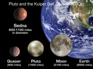
At present there are three dwarf planets by the definition of IAU. (Ceres: D~940km , Pluto: D~2300km, Eris: D~ 2400km) • Some papers have considered the effect of Pluto on the Plutinos. (Yu & Tremaine 1999; Nesvorny & Roig 2000) • We would like to know the gravitational influence of Eris on the Kuiper belt objects.
a=67 AU, e=0.44, i=440. • T=557 years. • mass=0.0028 ME, diameter=2400 km.
Although we don’t know where Eris was formed and how long Eris has stayed in the present orbit, but Eris should have some influence on the Kuiper belt. • The coagulation model (ex: Kenyon et al. 2007) implies that Eris-size objects were formed in a more massive disk (~30ME) with low e and i (e, i~10-3) planetesimals. • Under the planet migration model (ex: Hahn & Malhotra 2005), the scattered disk objects originated from low e, low i and smaller a orbitdue to Neptune’s migration. The migration timescale of Neptune is about 10 Myr. Therefore Eris-size objects may leave disk between 10 Myr to 4.5 Gyr.
The mass of Eris to the total mass of KBOs is about 0.1 (0.0028/0.03; Soter 2007) hence Eris may still collide and scatter with many other KBOs.
The main belt isnoteccentricity enough. • Absence of higher order resonance. (ex: 5:2) • High inclination KBOs are deficient. • Simulation: # of (3:2+2:1) / # of MB~2. Observation: # of (3:2+2:1) / # of MB~0.06.
We consider the Sun-Neptune-Eris-particle system in the late stage of planet migration model (the last several hundreds Myrs) and assume Eris at present orbit.
Sun-Neptune-Eris-Particle system N E S P
P η E y x N nt S ξ
For Eris: Jacobi constant
Numerical method • We used Runge-Kutta-Fehlberg method to solve the differential equations. This method combines 4th and 5th order Runge-Kutta method to choose a suitable step size for each step. • We did some modification in the step size determination in order to have a more significant criterion to choose the step size.
y y = f(t,y) RK5 yi+1 RK4 yi t hi
y y = f(t,y) ∆ RK4 yi+1 X RK4 □ yi t hi qhi R ≡ | ∆ | / (| X|+ | □ |) < TOL
The initial conditions: Neptune: a=30.07AU (1); e=0.0; θ=0.0 Eris: a=67.73AU (2.252); e=0.44; ω=0.0; θ=0.0 50 test particles in 3:2 mean motion resonance: a=39.4 ± 0.3 AU (1.31 ± 0.01); e=0.0,0.1,0.2,0.3,0.4; randomly assign ω,θ. 50 test particles in 2:1 mean motion resonance: a=47.7 ± 0.3 AU (1.59 ± 0.01); e=0.0,0.1,0.2,0.3,0.4; randomly assign ω,θ. 50 test particles in main belt: a=40.3 – 46.8AU (1.34 – 1.56); e=0.0,0.1; randomly assign ω,θ.
t0=0, tf=106TN (TN=165 yr) ∆tout=102TN ∆tmax=10-1TN, ∆tmin=10-20TN TOL=10-12 • The criterions for stopping the program: when r < 5AU or r > 1000AU when the particle collides with Neptune when the particle collides with Eris when t=tf
3to2: TS=438 yr 2to1: TS=845 yr
There two reasons cause the number of surviving particles of 3 :2 smaller than that of 2:1. One is that the synodic period of 3:2 is smaller than that of 2:1. Another is that the q=30 AU line in the a-e diagram crosses more region in 3:2 than that in 2:1 mean motion resonance.
# in 3to2: 13 # in MB: 57 # in 2to1: 21 (3to2+2to1)/MB = 0.6
Next Step • Construct three dimensional model. • Run more particles to enhance the statistical significance. From estimation of Hahn 2005 there are ~ 105 KBOs in the Kuiper belt. How many particles I will use depends on the computing sources. • Consider more Eris-size objects. How many? How to choose initial conditions? I am still thinking…….. Thank you ^^….. Any comment or suggestion?