Download
1 / 56
570 likes | 651 Vues
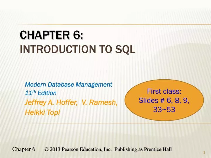
First class: Slides # 6, 8, 9 , 33~53. Modern Database Management 11 th Edition Jeffrey A. Hoffer, V. Ramesh, Heikki Topi. Chapter 6: Introduction to SQL. Objectives. Define terms Define a database using SQL data definition language Write single table queries using SQL

E N D
First class: Slides # 6, 8, 9, 33~53 Modern Database Management 11th Edition Jeffrey A. Hoffer, V. Ramesh, HeikkiTopi Chapter 6:Introduction to SQL
Objectives • Define terms • Define a database using SQL data definition language • Write single table queries using SQL • Establish referential integrity using SQL
SQL Overview • Structured Query Language • The standard for relational database management systems (RDBMS) • RDBMS: A database management system that manages data as a collection of tables in which all relationships are represented by common values in related tables
History of SQL • 1970–E. Codd develops relational database concept • 1974-1979–System R with Sequel (later SQL) created at IBM Research Lab • 1979–Oracle markets first relational DB with SQL • 1986–ANSI SQL standard released • 1989, 1992, 1999, 2003–Major ANSI standard updates • Current–SQL is supported by most major database vendors
Purpose of SQL Standard • Specify syntax/semantics for data definition and manipulation • Define data structures and basic operations • Enable portability of database definition and application modules • Specify minimal (level 1) and complete (level 2) standards • Allow for later growth/enhancement to standard
SQL Environment • Catalog • A set of schemas that constitute the description of a database • Schema • The structure that contains descriptions of objects created by a user (base tables, views, constraints) • Data Definition Language (DDL) • Commands that define a database, including creating, altering, and dropping tables and establishing constraints • Data Manipulation Language (DML) – our focus • Commands that maintain and query a database • Data Control Language (DCL) • Commands that control a database, including administering privileges and committing data
Figure 6-1 A simplified schematic of a typical SQL environment, as described by the SQL: 200n standard
Display order can be specified here 1 2 3 4 5 6 SELECT Major, AVERAGE(GPA) , ExpGraduateYr WHERE ExpGraduateYr = “2015” GROUP BY Major HAVING AVERAGE(GPA) >=3.0 ORDER BY Major Fig 6-2 Query syntax Cond for records Cond for groups Sequence! Just a quick example to show sequence of clauses
Figure 6-4 DDL, DML, DCL, and the database development process
SQL Database Definition • Data Definition Language (DDL) • Major CREATE statements: • CREATE SCHEMA–defines a portion of the database owned by a particular user • CREATE TABLE–defines a new table and its columns • CREATE VIEW–defines a logical table from one or more tables or views • Other CREATE statements: CHARACTER SET, COLLATION, TRANSLATION, ASSERTION, DOMAIN
Steps in table creation: • Identify data types for attributes • Identify columns that can and cannot be null • Identify columns that must be unique (candidate keys) • Identify primary key–foreign key mates • Determine default values • Identify constraints on columns (domain specifications) • Create the table and associated indexes Table Creation Figure 6-5 General syntax for CREATE TABLE statement used in data definition language
The following slides create tables for this enterprise data model (from Chapter 1, Figure 1-3)
14 Figure 6-3: sample PVFC data
Figure 6-6 SQL database definition commands for Pine Valley Furniture Company (Oracle 11g) Overall table definitions
Defining attributes and their data types Primary keys can never have NULL values Constraint name Cnstr Type Field
Non-nullable specifications composite key Some primary keys are composite– composed of multiple attributes
Controlling the values in attributes Default value Domain constraint validation rule
Identifying foreign keys and establishing relationships Primary key of parent table Foreign key of dependent table Constraint name CnstrntType Field REFERENCESTbl(Key)
Data Integrity Controls • Referential integrity–constraint that ensures that foreign key values of a table must match primary key values of a related table in 1:M relationships • Restricting: • Deletes of primary records • Updates of primary records • Inserts of dependent records
Figure 6-7 Ensuring data integrity through updates Relational integrity is enforced via the primary-key to foreign-key match
Changing Tables • ALTER TABLE statement allows you to change column specifications: • Table Actions: • Example (adding a new column with a default value): ADD COLUMN Name Type Default
Removing Tables • DROP TABLE statement allows you to remove tables from your schema: • DROP TABLE CUSTOMER_T
Insert Statement • Adds one or more rows to a table • Inserting into a table • VALUE – “s” Sequence!!! • Inserting a record that has some null attributes requires identifying the fields that actually get data INSERT INTO TableVALUES (value-list) (field-list) VALUES (value-list)
Insert Statement (cont) • Inserting from another table • A SUBSET from another table Interpretation?
Delete Statement • Removes rows from a table • Delete certain rows • DELETE FROM CUSTOMER_T WHERE CUSTOMERSTATE = ‘HI’; • Delete all rows • DELETE FROM CUSTOMER_T; • Careful!!!
Update Statement • Modifies data in existing rows • Note: the WHERE clause may be a subquery (Chap 7) • UPDATE Table-name • SET Attribute = Value • WHERE Criteria-to-apply-the-update
ALTER: changing the columns of the table • ALTER TABLE CUSTOMER_T ADD field… • INSERT: adding records based on the existing table • INSERT INTO CUSTOME_T VALUES (… ) • UPDATE: changing the values of some fields in existing records • UPDATE CUSTOMER_T SET field = value …WHERE… Comparison of ALTER, INSERT, and UPDATE
29 Recap of “three modifications”
Merge Statement Interpretation? Makes it easier to update a table…allows combination of Insert and Update in one statement Useful for updating master tables with new data
Schema Definition • Control processing/storage efficiency: • Choice of indexes • File organizations for base tables • File organizations for indexes • Data clustering • Statistics maintenance • Creating indexes • Speed up random/sequential access to base table data • Example • CREATE INDEX NAME_IDX ON CUSTOMER_T(CUSTOMERNAME) • This makes an index for the CUSTOMERNAME field of the CUSTOMER_T table
This is the CENTER section of the chapter, and the CENTER of this course Many slides contain multiple points of concepts/skills – do NOT miss the text, and play attention to color code Query: select statement
SELECT Example • Find products with standard price less than $275 Every SESLECT statement returns a result table - Can be used as part of another query SELECT DISTINCT: no duplicate rows SELECT * : all columns selected Table 6-3: Comparison Operators in SQL
SELECT Example Using Alias The two alias have very different usage … • Alias is an alternative column or table name SELECT CUST.CUSTOMER_NAME AS NAME, CUST.CUSTOMER_ADDRESS FROM CUSTOMER_V [AS] CUST WHERE NAME = ‘Home Furnishings’; Note1: Specifying source table, P. 262 Note2: Use of alias, P. 263
P. 264 • ProductStandardPrice*1.1 AS Plus10Percent • What does it look like which contents we learned in Access (in IS 312)? • Observe the result on P. 264 35 Using expressions (PP. 263-264)
More functions: P. 264~5 SELECT Example Using a Function • Using the COUNT aggregate function to find totals SELECT COUNT(*) FROM ORDERLINE_T WHERE ORDERID = 1004; Note 1: SELECT PRODUCT_ID, COUNT(*) FROM ORDER_LINE_V WHERE ORDER_ID = 1004; Note 2: COUNT (*) and COUNT - different P. 265 More exmpl: P. 266
SELECT Example Using functions • What is average standard price for each [examine!!] product in inventory? SELECT AVG (STANDARD_PRICE)AS AVERAGE FROM PROCUCT_V; • AVG, COUNT, MAX, MIN, SUM; • LN, EXP, POWER, SQRT • More functions – P. 264 • **Issues about set value and aggregates: 265-6** • Wildcards: 267, top • Null values, 268, top
Last line on P. 265: SQL cannot return both a row value (such as ID) and a set value (such as COUNT/AVG/SUM of a group); • users must run two separate queries, one that returns row info and one that returns set info • SELECT S_ID FROM STUDENT √ • SELECT AVG(GPA) FROM STUDENT √ • SELECT S_ID, AVG(GPA) FROM STUDENT Χ 38 Issues about set value and aggregates One of the above is not legitimate
SELECT Example–Boolean Operators • AND, OR, and NOT Operators for customizing conditions in WHERE clause Note: the LIKE operator allows you to compare strings using wildcards. For example, the % wildcard in ‘%Desk’ indicates that all strings that have any number of characters preceding the word “Desk” will be allowed.
SELECT Example–Boolean Operators • With parentheses…these override the normal precedence of Boolean operators Note: by default, the AND operator takes precedence over the OR operator. With parentheses, you can make the OR take place before the AND.
SELECT Example– Using distinct values • Compare: SELECT ORDER_ID FROM ORDER_LINE_V; and – SELECT DISTINCT ORDER_ID FROM ORDER_LINE_V; But: SELECT DISTINCT ORDER_ID, ORDER_QUANTITY FROM ORDER_LINE_V; Compare three figures on 272 & 273
SELECT Example – Sorting Results with the ORDER BY Clause • Sort the results first by STATE, and then within a state by the CUSTOMER NAME Can order by multiple fields: primary sort, 2ndry sort, … Note: the IN operator in this example allows you to include rows whose CustomerState value is either FL, TX, CA, or HI. It is more efficient than separate OR conditions. The opposite is NOT IN
SELECT Example– Categorizing Results Using the GROUP BY Clause • For use with aggregate functions • Scalar aggregate: single value returned from SQL query with aggregate function – those in PP. 264~266 (aggregate of whole table) • Vector aggregate: multiple values returned from SQL query with aggregate function (via GROUP BY) P. 275 near bottom: Each column referenced in the SELECT statement must be referenced in the GROUP BY clause; if not, it must be used as an argument for an aggregate Fn One value for a group “vector” Result: P. 275
SELECT S_ID FROM STUDENT SELECT MAJOR, AVG(GPA) FROM STUDENT GROUP BY MAJOR SELECT S_ID, AVG(GPA) FROM STUDENT GROUP BY MAJOR SELECT COUNT(S_ID), AVG(GPA) FROM STUDENT GROUP BY MAJOR 46 single-value fields vsaggregate functions One of the above is not legitimate. Compare Slide #39
SELECT Example– Qualifying Results by Categories Using the HAVING Clause • For use with GROUP BY Like a WHERE clause, but it operates on groups (categories), not on individual rows. Here, only those groups with total numbers greater than 1 will be included in final result. See 275-276
SELECT Statement with Group by • Used for queries on single or multiple tables • Clauses of the SELECT statement: (Sequence!!) • SELECT • List the columns (and expressions) that should be returned from the query • FROM • Indicate the table(s) or view(s) from which data will be obtained • WHERE • Indicate the conditions under which a row will be included in the result • GROUP BY • Indicate categorization of results • HAVING • Indicate the conditions under which a category (group) will be included • ORDER BY • Sorts the result according to specified criteria Can have multiple sorts – primary, 2ndry, … Read closely PP. 275-276
Figure 6-10 • SQL statement processing order (adapted from van der Lans, 2006 p.100)
HAVING clause • The HAVING clause acts like a WHERE clause, but it identifies groups that meet a criterion, rather than rows. • Therefore, you will usually see a HAVING clause … • WHERE qualifies a set of rows, while HAVING qualifies a set of … Interpretation: example on P. 276