Download
1 / 17
170 likes | 317 Vues
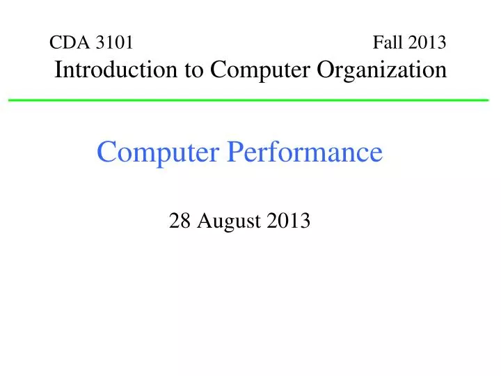
CDA 3101 Fall 2013 Introduction to Computer Organization. Computer Performance 28 August 2013. Overview. Performance evaluation Limitations Metrics Processor performance equation Performance evaluation reports Amdahl’s law.

E N D
CDA 3101 Fall 2013Introduction to Computer Organization Computer Performance 28 August 2013
Overview • Performance evaluation • Limitations • Metrics • Processor performance equation • Performance evaluation reports • Amdahl’s law
Performance Evaluation Program Compiler ISA CPI Microarchitecture Hardware Manufacturing
Performance Evaluation Concepts • Computer performance evaluation is based on: • Throughput (bits per second) • Response time (a.k.a. execution time, elapsed time) • Component- and system-level performance • Processor performance evaluation • Based on execution time of a program: PerformanceX = 1/ Execution timeX Relative performance: n = PerformanceX / PerformanceY n > 1 => X is n times faster than Y • Terminology • Improve performance = increase performance • Improve execution time = decrease execution time
Example • Impact on throughput and response time of: • Using a faster processor • Decrease in response time • Increase in throughput • Adding more processors to a system • Increase in throughput • Decrease in response time (if overhead is low) • In Massively Parallel Processors (MPP) • In Symmetric Multiprocessing Processors (SMP) • Only if additional processors reduce queue time
Measuring Performance Components of the execution time of a program: • CPU execution time • User CPU time • System CPU time • I/O time • Time spent running other programs Unix time command time cc prog.c 9.7u 1.5s 20 56% 9.7u = 9.7 sec User CPU time 1.5s = 1.5 sec System CPU time 20 = Total Elapsed Time 56% = Percent CPU time
CPU Performance Equation • CPU time = CPU clock cycles * cycle time = CPU clock cycles / clock rate • CPU clock cycles = IC * CPI • IC: instruction count (number of instructions per program) • CPI: average cycles per instruction CPU time = IC * CPI * cycle time seconds instructions clock cycles seconds program program instruction clock cycle • CPU clock cycles = Σi (CPIi * ICi) • ICi : count of instructions of class i • CPIi : cycles that takes to execute instructions of class i * * =
Scope of Performance Sources CPU time =IC* CPI *Cycle time Program Compiler ISA Microarchitecture Hardware Abstraction level interdependence
Example 1 • A program runs in 10 secs on a 2.0 GHz processor. A designer wants to build a new computer that can run the program in 6 secs by increasing the clock frequency. However the average “new” CPI will be 1.2 times higher. • What faster clock rate should the designer use? 10 IC * CPI / 2 GHz (current exec. time) 6 IC * 1.2 CPI / X GHz (target execution time) Solve for X, to obtainX = ___ GHz =
Example 2 • Comparing two compiler code segments • Which code sequence executes the most instructions? • Which will be faster? S1 = 2 . 1 + 1 . 2 + 2 . 3 = 10 cyc S2 = 4. 1 + 1 . 2 + 1 . 3 = 9 cyc
Components of the CPU Equation • IC Instruction count • Compiler • Instruction set simulator • Execution-based monitoring (profiling) • CPI if pipelined execution is used CPIi = PipelineCPIi + Memory CPIi • Clock cycle time • Timing estimators or verifiers (complete design) • Target cycle time
Performance Evaluation Programs • Ideal situation: known programs (workload) • Benchmarks • Real programs • Kernels • Toy benchmarks • Synthetic benchmarks • Risk: adjust design to benchmark requirements • (partial) solution: use real programs • Engineering or scientific applications • Software development tools • Transaction processing • Office applications Convenience Realism
Performance Reports • Reproducibility • Include hardware / software configuration • Evaluation process conditions • Summarizing performance • Total time: CPU time + I/O time + Other time • Arithmetic mean: AM = 1/n * Σ exec timei • Harmonic mean: HM = n / Σ (1/ratei) • Weighted mean: WM = Σ wi * exec timei • Geometric mean: GM = (Π exec time ratioi)1/n GM (Xi) Xi GM (Yi) Yi Important Stuff =
Arithmetic and Geometric Means A B C P1 1 10 20 P2 1000 100 20 Execution time (in seconds) machines: A, B, and C programs: P1 and P2
Amdahl’s Law Execution time before improvement Execution time after improvement • Law of diminishing returns Speedup = Example: Two factors - F1: 75% improve, F2: 50% improve F1 F2 1 (1 - fraction enhanced) + (fraction enhanced/factor of improvement) Speedup =
Example • A program runs in 10 seconds • What is the speedup after a faster floating point unit is incorporated? 1 Speedup = (1 – Fraction FP) + FractionFP 5 1 Speedup = 0.5 0.5 + FP factor of improvement
Conclusions • Many different performance data • CPU time, I/O time, Other time, Total time • Select best presentation method • Arithmetic mean for execution times • Geometric mean for performance ratios • Watch out for Amdahl’s Law • Diminishing returns w/ improved performance • Impacts of development Co$t