Download
1 / 50
530 likes | 991 Vues
Chapter 3 Heuristic Search Techniques. Contents. A framework for describing search methods is provided and several general purpose search techniques are discussed. All are varieties of Heuristic Search: Generate and test Hill Climbing Best First Search Problem Reduction

E N D
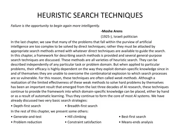
Contents • A framework for describing search methods is provided and several general purpose search techniques are discussed. • All are varieties of Heuristic Search: • Generate and test • Hill Climbing • Best First Search • Problem Reduction • Constraint Satisfaction • Means-ends analysis
Generate-and-Test • Algorithm: • Generate a possible solution. For some problems, this means generating a particular point in the problem space. For others it means generating a path from a start state • Test to see if this is actually a solution by comparing the chosen point or the endpoint of the chosen path to the set of acceptable goal states. • If a solution has been found, quit, Otherwise return to step 1.
Generate-and-Test • It is a depth first search procedure since complete solutions must be generated before they can be tested. • In its most systematic form, it is simply an exhaustive search of the problem space. • Operate by generating solutions randomly. • Also called as British Museum algorithm • If a sufficient number of monkeys were placed in front of a set of typewriters, and left alone long enough, then they would eventually produce all the works of shakespeare. • Dendral: which infers the struture of organic compounds using NMR spectrogram. It uses plan-generate-test.
Hill Climbing • Is a variant of generate-and test in which feedback from the test procedure is used to help the generator decide which direction to move in search space. • The test function is augmented with a heuristic function that provides an estimate of how close a given state is to the goal state. • Computation of heuristic function can be done with negligible amount of computation. • Hill climbing is often used when a good heuristic function is available for evaluating states but when no other useful knowledge is available.
Simple Hill Climbing • Algorithm: • Evaluate the initial state. If it is also goal state, then return it and quit. Otherwise continue with the initial state as the current state. • Loop until a solution is found or until there are no new operators left to be applied in the current state: • Select an operator that has not yet been applied to the current state and apply it to produce a new state • Evaluate the new state • If it is the goal state, then return it and quit. • If it is not a goal state but it is better than the current state, then make it the current state. • If it is not better than the current state, then continue in the loop.
Simple Hill Climbing • The key difference between Simple Hill climbing and Generate-and-test is the use of evaluation function as a way to inject task specific knowledge into the control process. • Is on state better than another ? For this algorithm to work, precise definition of better must be provided.
Steepest-Ascent Hill Climbing • This is a variation of simple hill climbing which considers all the moves from the current state and selects the best one as the next state. • Also known as Gradient search
Algorithm: Steepest-Ascent Hill Climbing • Evaluate the initial state. If it is also a goal state, then return it and quit. Otherwise, continue with the initial state as the current state. • Loop until a solution is found or until a complete iteration produces no change to current state: • Let SUCC be a state such that any possible successor of the current state will be better than SUCC • For each operator that applies to the current state do: • Apply the operator and generate a new state • Evaluate the new state. If is is a goal state, then return it and quit. If not, compare it to SUCC. If it is better, then set SUCC to this state. If it is not better, leave SUCC alone. • If the SUCC is better than the current state, then set current state to SYCC,
: Hill-climbing This simple policy has three well-known drawbacks:1. Local Maxima: a local maximum as opposed to global maximum.2. Plateaus: An area of the search space where evaluation function is flat, thus requiring random walk.3. Ridge: Where there are steep slopes and the search direction is not towards the top but towards the side. (a) (b) (c) Figure 5.9 Local maxima, Plateaus and ridge situation for Hill Climbing
Hill-climbing • In each of the previous cases (local maxima, plateaus & ridge), the algorithm reaches a point at which no progress is being made. • A solution is to do a random-restart hill-climbing - where random initial states are generated, running each until it halts or makes no discernible progress. The best result is then chosen. Figure 5.10 Random-restart hill-climbing (6 initial values) for 5.9(a)
Simulated Annealing • A alternative to a random-restart hill-climbing when stuck on a local maximum is to do a ‘reverse walk’ to escape the local maximum. • This is the idea of simulated annealing. • The term simulated annealing derives from the roughly analogous physical process of heating and then slowly cooling a substance to obtain a strong crystalline structure. • The simulated annealing process lowers the temperature by slow stages until the system ``freezes" and no further changes occur.
Simulated Annealing Figure 5.11 Simulated Annealing Demo (http://www.taygeta.com/annealing/demo1.html)
Simulated Annealing • Probability of transition to higher energy state is given by function: • P = e –∆E/kt Where ∆E is the positive change in the energy level T is the temperature K is Boltzmann constant.
Differences • The algorithm for simulated annealing is slightly different from the simple-hill climbing procedure. The three differences are: • The annealing schedule must be maintained • Moves to worse states may be accepted • It is good idea to maintain, in addition to the current state, the best state found so far.
Algorithm: Simulate Annealing • Evaluate the initial state. If it is also a goal state, then return it and quit. Otherwise, continue with the initial state as the current state. • Initialize BEST-SO-FAR to the current state. • Initialize T according to the annealing schedule • Loop until a solution is found or until there are no new operators left to be applied in the current state. • Select an operator that has not yet been applied to the current state and apply it to produce a new state. • Evaluate the new state. Compute: • ∆E = ( value of current ) – ( value of new state) • If the new state is a goal state, then return it and quit. • If it is a goal state but is better than the current state, then make it the current state. Also set BEST-SO-FAR to this new state. • If it is not better than the current state, then make it the current state with probability p’ as defined above. This step is usually implemented by invoking a random number generator to produce a number in the range [0, 1]. If the number is less than p’, then the move is accepted. Otherwise, do nothing. • Revise T as necessary according to the annealing schedule • Return BEST-SO-FAR as the answer
Simulate Annealing: Implementation • It is necessary to select an annealing schedule which has three components: • Initial value to be used for temperature • Criteria that will be used to decide when the temperature will be reduced • Amount by which the temperature will be reduced.
Best First Search • Combines the advantages of bith DFS and BFS into a single method. • DFS is good because it allows a solution to be found without all competing branches having to be expanded. • BFS is good because it does not get branches on dead end paths. • One way of combining the tow is to follow a single path at a time, but switch paths whenever some competing path looks more promising than the current one does.
BFS • At each step of the BFS search process, we select the most promising of the nodes we have generated so far. • This is done by applying an appropriate heuristic function to each of them. • We then expand the chosen node by using the rules to generate its successors • Similar to Steepest ascent hill climbing with two exceptions: • In hill climbing, one move is selected and all the others are rejected, never to be reconsidered. This produces the straightline behaviour that is characteristic of hill climbing. • In BFS, one move is selected, but the others are kept around so that they can be revisited later if the selected path becomes less promising. Further, the best available state is selected in the BFS, even if that state has a value that is lower than the value of the state that was just explored. This contrasts with hill climbing, which will stop if there are no successor states with better values than the current state.
OR-graph • It is sometimes important to search graphs so that duplicate paths will not be pursued. • An algorithm to do this will operate by searching a directed graph in which each node represents a point in problem space. • Each node will contain: • Description of problem state it represents • Indication of how promising it is • Parent link that points back to the best node from which it came • List of nodes that were generated from it • Parent link will make it possible to recover the path to the goal once the goal is found. • The list of successors will make it possible, if a better path is found to an already existing node, to propagate the improvement down to its successors. • This is called OR-graph, since each of its branhes represents an alternative problem solving path
Implementation of OR graphs • We need two lists of nodes: • OPEN – nodes that have been generated and have had the heuristic function applied to them but which have not yet been examined. OPEN is actually a priority queue in which the elements with the highest priority are those with the most promising value of the heuristic function. • CLOSED- nodes that have already been examined. We need to keep these nodes in memory if we want to search a graph rather than a tree, since whenver a new node is generated, we need to check whether it has been generated before.
Algorithm: BFS • Start with OPEN containing just the initial state • Until a goal is found or there are no nodes left on OPEN do: • Pick the best node on OPEN • Generate its successors • For each successor do: • If it has not been generated before, evaluate it, add it to OPEN, and record its parent. • If it has been generated before, change the parent if this new path is better than the previous one. In that case, update the cost of getting to this node and to any successors that this node may already have.
BFS : simple explanation • It proceeds in steps, expanding one node at each step, until it generates a node that corresponds to a goal state. • At each step, it picks the most promising of the nodes that have so far been generated but not expanded. • It generates the successors of the chosen node, applies the heuristic function to them, and adds them to the list of open nodes, after checking to see if any of them have been generated before. • By doing this check, we can guarantee that each node only appears once in the graph, although many nodes may point to it as a successor.
A A A A B B B B C C C C D D D D 5 5 5 5 1 1 1 1 3 3 3 3 E E E F F F 4 4 4 6 6 6 G G H H 6 6 5 5 BFS Step 2 Step 3 Step 1 A Step 5 Step 4 A 2 A 1
A* Algorithm • BFS is a simplification of A* Algorithm • Presented by Hart et al • Algorithm uses: • f’: Heuristic function that estimates the merits of each node we generate. This is sum of two components, g and h’ and f’ represents an estimate of the cost of getting from the initial state to a goal state along with the path that generated the current node. • g : The function g is a measure of the cost of getting from initial state to the current node. • h’ : The function h’ is an estimate of the additional cost of getting from the current node to a goal state. • OPEN • CLOSED
A* Algorithm • Start with OPEN containing only initial node. Set that node’s g value to 0, its h’ value to whatever it is, and its f’ value to h’+0 or h’. Set CLOSED to empty list. • Until a goal node is found, repeat the following procedure: If there are no nodes on OPEN, report failure. Otherwise picj the node on OPEN with the lowest f’ value. Call it BESTNODE. Remove it from OPEN. Place it in CLOSED. See if the BESTNODE is a goal state. If so exit and report a solution. Otherwise, generate the successors of BESTNODE but do not set the BESTNODE to point to them yet.
A* Algorithm ( contd) • For each of the SUCCESSOR, do the following: • Set SUCCESSOR to point back to BESTNODE. These backwards links will make it possible to recover the path once a solution is found. • Compute g(SUCCESSOR) = g(BESTNODE) + the cost of getting from BESTNODE to SUCCESSOR • See if SUCCESSOR is the same as any node on OPEN. If so call the node OLD. • If SUCCESSOR was not on OPEN, see if it is on CLOSED. If so, call the node on CLOSED OLD and add OLD to the list of BESTNODE’s successors. • If SUCCESSOR was not already on either OPEN or CLOSED, then put it on OPEN and add it to the list of BESTNODE’s successors. Compute f’(SUCCESSOR) = g(SUCCESSOR) + h’(SUCCESSOR)
Observations about A* • Role of g function: This lets us choose which node to expand next on the basis of not only of how good the node itself looks, but also on the basis of how good the path to the node was. • h’, the distance of a node to the goal.If h’ is a perfect estimator of h, then A* will converge immediately to the goal with no search.
Gracefull Decay of Admissibility • If h’ rarely overestimates h by more than δ, then A* algorithm will rarely find a solution whose cost is more than δ greater than the cost of the optimal solution. • Under certain conditions, the A* algorithm can be shown to be optimal in that it generates the fewest nodes in the process of finding a solution to a problem.
Agendas • An Agenda is a list of tasks a system could perform. • Associated with each task there are usually two things: • A list of reasons why the task is being proposed (justification) • Rating representing the overall weight of evidence suggesting that the task would be useful.
Algorithm: Agenda driven Search • Do until a goal state is reached or the agenda is empty: • Choose the most promising task from the agenda. • Execute the task by devoting to it the number of resources determined by its importance. The important resources to consider are time and space. Executing the task will probably generate additional tasks (successor nodes). For each of them do the followings: • See if it is already on the agenda. If so, then see if this same reason for doing it is already on its list of justifications. If so, ignore this current evidence. If this justification was not already present, add it to the list. If the task was not on the agenda, insert it. • Compute the new task’s rating, combining the evidence from all its justifications. Not all justifications need have equal weight. It is often useful to associate with each justification a measure of how strong the reason it is. These measures are then combined at this step to produce an overall rating for the task.
Chatbot Person: I don’t want to read any more about china. Give me something else. Computer: OK. What else are you interested in? Person: How about Italy? I think I’d find Italy interesting. Computer : What things about Italy are you interested in reading about? Person: I think I’d like to start with its history. Computer: why don’t you want to read any more about China?
Example for Agenda: AM • Mathematics discovery program developed by Lenat ( 77, 82) • AM was given small set of starting facts about number theory and a set of operators it could use to develop new ideas. • These operators included such things as “ Find examples of a concept you already know”. • AM’s goal was to generate new “interesting” Mathematical concepts. • It succeeded in discovering such things as prime numbers and Goldbach’s conjecture. • AM used task agenda.
AND-OR graphs • AND-OR graph (or tree) is useful for representing the solution of problems that can be solved by decomposing them into a set of smaller problems, all of which must then be solved. • One AND arc may point to any number of successor nodes, all of which must be solved in order for the arc to point to a solution. Goal: Acquire TV Set Goal: Steal a TV Set Goal: Buy TV Set Goal: Earn some money
A A 38 9 B C D 3 4 5 B C D 17 27 9 E F G H I J 5 3 4 15 10 10 AND-OR graph examples
Problem Reduction • FUTILITY is chosen to correspond to a threshold such than any solution with a cost above it is too expensive to be practical, even if it could ever be found. Algorithm : Problem Reduction • Initialize the graph to the starting node. • Loop until the starting node is labeled SOLVED or until its cost goes above FUTILITY: • Traverse the graph, starting at the initial node and following the current best path, and accumulate the set of nodes that are on that path and have not yet been expanded or labeled as solved. • Pick one of these nodes and expand it. If there are no successors, assign FUTILITY as the value of this node. Otherwise, add its successors to the graph and for each of them compute f’. If f’ of any node is 0, mark that node as SOLVED. • Change the f’ estimate of the newly expanded node to reflect the new information provided by its successors. Propagate this change backward through the graph. This propagation of revised cost estimates back up the tree was not necessary in the BFS algorithm because only unexpanded nodes were examined. But now expanded nodes must be reexamined so that the best current path can be selected.
Constraint Satisfaction • Constraint Satisfaction problems in AI have goal of discovering some problem state that satisfies a given set of constraints. • Design tasks can be viewed as constraint satisfaction problems in which a design must be created within fixed limits on time, cost, and materials. • Constraint satisfaction is a search procedure that operates in a space of constraint sets. The initial state contains the constraints that are originally given in the problem description. A goal state is any state that has been constrained “enough” where “enough”must be defined for each problem. For example, in cryptarithmetic, enough means that each letter has been assigned a unique numeric value. • Constraint Satisfaction is a two step process: • First constraints are discovered and propagated as far as possible throughout the system. • Then if there still not a solution, search begins. A guess about something is made and added as a new constraint.
Algorithm: Constraint Satisfaction • Propagate available constraints. To do this first set OPEN to set of all objects that must have values assigned to them in a complete solution. Then do until an inconsistency is detected or until OPEN is empty: • Select an object OB from OPEN. Strengthen as much as possible the set of constraints that apply to OB. • If this set is different from the set that was assigned the last time OB was examined or if this is the first time OB has been examined, then add to OPEN all objects that share any constraints with OB. • Remove OB from OPEN. • If the union of the constraints discovered above defines a solution, then quit and report the solution. • If the union of the constraints discovered above defines a contradiction, then return the failure. • If neither of the above occurs, then it is necessary to make a guess at something in order to proceed. To do this loop until a solution is found or all possible solutions have been eliminated: • Select an object whose value is not yet determined and select a way of strengthening the constraints on that object. • Recursively invoke constraint satisfaction with the current set of constraints augmented by strengthening constraint just selected.
Constraint Satisfaction: Example • Cryptarithmetic Problem: SEND +MORE ----------- MONEY Initial State: • No two letters have the same value • The sums of the digits must be as shown in the problem Goal State: • All letters have been assigned a digit in such a way that all the initial constraints are satisfied.
Cryptasithmetic Problem: Constraint Satisfaction • The solution process proceeds in cycles. At each cycle, two significant things are done: • Constraints are propagated by using rules that correspond to the properties of arithmetic. • A value is guessed for some letter whose value is not yet determined. A few Heuristics can help to select the best guess to try first: • If there is a letter that has only two possible values and other with six possible values, there is a better chance of guessing right on the first than on the second. • Another useful Heuristic is that if there is a letter that participates in many constraints then it is a good idea to prefer it to a letter that participates in a few.
Solving a Cryptarithmetic Problem Initial state SEND +MORE ------------- MONEY M=1 S= 8 or 9 O = 0 or 1 -> O =0 N= E or E+1 -> N= E+1 C2 = 1 N+R >8 E<> 9 E=2 N=3 R= 8 or 9 2+D = Y or 2+D = 10 +Y C1= 0 C1= 1 2+D =Y N+R = 10+E R =9 S =8 2+D = 10 +Y D = 8+Y D = 8 or 9 D=8 D=9 Y= 0 ; Conflict Y =1 ; Conflict
Means-Ends Analysis(MEA) • We have presented collection of strategies that can reason either forward or backward, but for a given problem, one direction or the other must be chosen. • A mixture of the two directions is appropriate. Such a mixed strategy would make it possible to solve the major parts of a problem first and then go back and solve the small problems that arise in “gluing” the big pieces together. • The technique of Means-Ends Analysis allows us to do that.
Algorithm: Means-Ends Analysis • Compare CURRENT to GOAL. If there if no difference between them then return. • Otherwise, select the most important difference and reduce it by doing the following until success of failure is signaled: • Select an as yet untried operator O that is applicable to the current difference. If there are no such operators, then signal failure. • Attempt to apply O to CURRENT. Generate descriptions of two states: O-START, a state in which O’s preconditions are satisfied and O-RESULT, the state that would result if O were applied in O-START. • If (FIRST-PART <- MEA( CURRENT, O-START)) and (LAST-PART <- MEA(O-RESULT, GOAL)) are successful, then signal success and return the result of concatenating FIRST-PART, O, and LAST-PART.
MEA: Operator Subgoaling • MEA process centers around the detection of differences between the current state and the goal state. • Once such a difference is isolated, an operator that can reduce the difference must be found. • If the operator cannot be applied to the current state, we set up a subproblem of getting to a state in which it can be applied. • The kind of backward chaining in which operators are selected and then subgoals are set up to establish the preconditions of the operators.
MEA: Progress B D C A Push Goal start D A B C E walk Pick up Put Down Place Pick Up Put Down Push Goal Start
Summary Four steps to design AI Problem solving: • Define the problem precisely. Specify the problem space, the operators for moving within the space, and the starting and goal state. • Analyze the problem to determine where it falls with respect to seven important issues. • Isolate and represent the task knowledge required • Choose problem solving technique and apply them to problem.
Summary • What the states in search spaces represent. Sometimes the states represent complete potential solutions. Sometimes they represent solutions that are partially specified. • How, at each stage of the search process, a state is selected for expansion. • How operators to be applied to that node are selected. • Whether an optimal solution can be guaranteed. • Whether a given state may end up being considered more than once. • How many state descriptions must be maintained throughout the search process. • Under what circumstances should a particular search path be abandoned.