Download
1 / 23
360 likes | 1.06k Vues
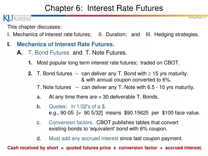
Chapter 6: Interest Rate Futures. This chapter discusses : I. Mechanics of interest rate futures ; II. Duration ; and III . Hedging strategies. I. Mechanics of Interest Rate Futures. A . T. Bond Futures and T . Note Futures.

E N D
Chapter 6: Interest Rate Futures This chapter discusses: I. Mechanics of interest rate futures; II. Duration; and III. Hedging strategies. I.Mechanics of Interest Rate Futures. A.T. Bond Futures and T. Note Futures. 1. Most popular long term interest rate futures; traded on CBOT. 2. T. Bond futures -- can deliver any T. Bond with 15 yrs maturity. & with annual coupon converted to 6%. T. Note futures -- can deliver any T. Note with 6.5 - 10 yrs maturity. a. At any time there are 30 deliverable T. Bonds. b. Quotes: in 1/32's of a $. e.g., 90-05 [= 90 5/32] means $90.15625 per $100 face value. c. Conversion factors. CBOT publishes tables that convert existing bonds to 'equivalent' bond with 6% coupon. d. Must add any accrued interest since last coupon payment. Cash received by short = quoted futures price x conversion factor + accrued interest.
I.A. T.Bond and T.Note Futures 3. Delivery options add value to short position. a. Can deliver on any day of delivery month. b. Can choose cheapest-to-deliver bond. i. If yields > 6%, deliver low coupon, long maturity bonds; (worth less) If yields < 6%, deliver high coupon, short maturity bonds. ii. If yield curve upward sloping, deliver long bonds; If yield curve downward sloping, deliver short bonds. iii. Some bonds sell for more than their theoretical value; e.g., low-coupon bonds; bonds where coupons can be stripped. These have abnormal demand & will not likely be cheapest to deliver. c. Wild card play (a timing option). On expiration day at CBOT, T.Bondfutures trading ends at 2 pm; T.Bondsthemselves trade until 4 pm. Short futures position can announce intent to deliver 8pm. If bond prices after 2 pm, can announce intent to deliver & then buy cheapest bond for delivery. Otherwise, wait till next day. d. NOTE: Delivery options are not free; Value is reflected in F (↓F).
I.A. T.Bond and T.Note Futures 4. Determining Futures Price applicable in a trade. a. Complicated by options held by short position re: choice of bond and timing of delivery. b. If the cheapest-to-deliver bond and date of delivery are known, then this is a futures on a security that pays a known income: F* = (S - I)erT c. Steps: i. Calculate cash price (S) of cheapest-to-deliver bond; ii. Calculate cash futures price (F) from equation above; iii. Apply the conversion factor to F in ii. iv. Calculate the quoted futures price from F in iii., by adding any accrued interest;
I.B. T.Bill and Eurodollar Futures Most popular short term interest rate futures. 1. T. Bill Futures (traded on CME). 2.Eurodollar Futures; (IMM & LIFFE). We’ll focus on this. a. Eurodollar -- U.S. $ deposited outside the U.S. b. Eurodollar rate -- LIBOR; i. Rate earned on ED deposited by one bank with another bank. ii. Determined by trading of deposits between banks on the Eurocurrency market. iii. 1-month LIBOR is rate offered by one bank to another on 1-month deposits at a given time. If variable rate loan charges 1-month LIBOR, then rate is reset to 1-month LIBOR at 1-month intervals, with interest paid in arrears. iv. Other analogous rates are 3-month & 6-month LIBOR.
I.B. T.Bill and Eurodollar Futures c. LIBOR is generally higher than corresponding T.Billrate. LIBOR is a commercial lending rate (not gov't borrowing). d. Eurodollar futures contract similar to T. Bill futures contract. e. Some important differences: i. T. Bill futures contract delivers a 90-day T. Bill. Eurodollar futures contract is settled in cash. ii. Final marking-to-market sets contract price equal to: VF = 10,000( 100 - .25R ), where R = quoted 90-day ED rate (LIBOR) at that time. iii. Note that this quoted ED rate is the actual 90-day rate on ED deposits with quarterly compounding -- not a discount rate. Hence, ED contract is a futures on an interest rate, while T.Billcontract is a futures on a T. Bill.
I.B. T.Bill and Eurodollar Futures 3.ED Futures Contract Characteristics: a. Underlying Asset – $1 MM ED deposit with 3-month maturity. b. ED rates quoted on interest-bearing basis, assuming 360-day year. c. Each ED futures contract represents $1 MM face value, ED deposits maturing 3 months after contract expiration. d. 40 different contracts trade at any point in time; contracts mature in Mar, Je, Sept, & Dec 10 years out. e. Settlement in cash; Price established by survey of current ED rates. f. ED futures trade according to an index quote (Q); Q = 100 - R, where R = quoted futures interest rate; e.g., If futures rate = R = 8.50%, then Q = 91.50, and interest outlay promised would be: (.0850) x ($1,000,000) x (90 / 360) = $21,250.
I.B. T.Bill and Eurodollar Futures g. Value of one ED futures contract = VF = 10,000 (100 - .25R), where R = quoted 90-day ED fwd rate (LIBOR) at that time. e.g., if quoted futures price is Q = 91.50, then R = 8.50, and VF = $10,000 [ 100 - .25 (100 - 91.50) ] = $10,000 [ 100 - .25 (8.50) ] = $10,000 [ 100 - 2.125 ] = $10,000 [ 97.875 ] = $978,750 ** VF = $1,000,000 - $21,250 (= $1,000,000 - interest outlay). h. Each basis point change in futures rate means a $25 change in value of the contract (interest outlay promised) : [ (.0001) x ($1,000,000) x (90 / 360) ] = $25. i. The futures is truly a futures on an interest rate. (The T.Bill futures is a futures on a 90-day T.Bill.)
I.B. T.Bill and Eurodollar Futures 4. Example: Long Hedge with ED futures for a Bank. Jan. 6: Bank expects to receive $1 MM payment on May 11 (4 months). Anticipates investing funds in 3-month ED deposits. Cash Market risk exposure: Bank would like to invest @ today’s ED rate, but won’t have funds for 4 months. If ED rate , bank will realize opportunity loss (will have to invest the $1 MM at lower ED rates). Long Hedge: Buy ED futures today (promise to deposit later @ R). Then if cash rates , futures rates (R) will & futures prices (Q) will . so long futures position will to offset opportunity losses in cash mkt. The best ED futures to buy is June contract; expires soonest after May 11. Jan. 6 May 11 June 14 |__________________________________________|_____________| $1 MM receivable due May 11. Cash: Plan to invest $1MM on May 11Invest the $1 MM in ED deposits. Futures: Buy 1 ED futures contract.Sell the futures contract.
I.B. T.Bill and Eurodollar Futures Data for example – Jan. 6: Cash market ED rate (LIBOR) = RS = 3.38% (S1 = 96.62) June ED futures rate (LIBOR) = RF = 3.85% (F1 = 96.15) ; Basis = (S1 - F1) = .47% May 11: Cash market ED rate = 3.03% (S2 = 96.97) June ED futures rate = 3.60% (F2 = 96.40) ; Basis = (S2 - F2) = .57% _______________________________________________________________________________ DateCash Market Futures Market Basis 1 / 6bank plans to invest $1MM bank buys 1 Je ED futures at cash rate = S0 = 3.38% at futures rate = R0 = 3.85%.47% 5 / 11bank invests $1MM in 3-mo ED bank sells 1 June ED futures at cash rate = S1 = 3.03% at futures rate = R1 = 3.60%.57% Netopport. loss = 3.38 - 3.03 = .35% futures gain = 3.85 - 3.60 = .25% change Effect(35) x ($25) = $875 (25) x ($25) = $625 .10% . Cumulative Investment Income: Interest @ 3.03% = $1,000,000 (.0303) (90/360) = $7,575 Profit from futures trades: = $625 Total: $8,200 Effective Return = [ $8,200 / $1,000,000 ] x (360 / 90) = 3.28% (10 bpworse than spot market = change in basis). This is basis risk.
II. Duration A measure of how long, on average, bondholder must wait to receive cash. -- A Zero-coupon bond maturing in n years has D = n; A Coupon-bearing bond maturing in n years has D < n; some cash received < n. A. Definition. 1.Assume: Today is t0. Bond pays coupons, ci, at times ti (1 i n). Then Bond price, B, and yield, y, are related: B = Σ ci e -y (ti) . n n┌─ ─┐ Duration: D = [ Σ tici e -y (ti) ] / B = Σ ti │ ci e -y (ti) / B │ n=1n=1└─ ─┘ 2. Notes: a. The term in brackets is NPV(payment at time ti) divided by bond price, B, which is NPV(all payments). b. Thus, D is weighted avg of times when payments are made with the weight for time ti a measure of how important the payment is (i.e., the proportion of B provided by the payment at time ti ). c. The weights sum to 1.
II.B. Derivation of Duration Formula 1. Digression: New Definition of Risk – “exposure” or Sensitivity to changes in underlying source of uncertainty. For example, consider the Market Model: Ri = αi + βiRM + εi: Risk = βi = dRi/ dRM(Sensitivity) n 2. Given formula for bond price: B = Σ ci e -y (ti), i=1 We are interested in the sensitivity of the bond price, B, to a change in yield, y : n B / y = - Σ (ti)ci e -y (ti) = -BD . i=1 ( Like the β of a stock – this is risk! )
II.B. Derivation of Duration Formula 3. Intuition: a. If we make a parallel shift in the yield curve, increasing all rates by Δy, this also increases all bond rates by Δy. b. Thus, bond prices will change by ΔB, where ΔB / Δy= -BD or ΔB = -BDΔyor ΔB / B = -DΔy c. Thus, % change in bond price = (duration) x (size of parallel shift in yield curve). ** Like the β of a stock portfolio – sensitivity or exposureto market. ** This relation enables hedger to assess the sensitivityof a bond to small changes in its yield. This information helps to hedge a bond portfolio.
II.C. Example - Calculating Bond Duration 1. Consider the following bond: Face Value = $100; C / F = 10% coupon (semi-annual payments of $5); n = 3 years maturity; y = 12% p.a.; (Note: coupon rate < mkt rate) _____________________________________________________________________ Time Payment PV Weight Time x Weight (ti) ci ci e -y (ti)Pvi B (ti) x Wi _____________________________________________________________________ 0.5 $5$4.709 .050 .025 1.0 $5$4.435 .047 .047 1.5 $5$4.176 .044 .066 2.0 $5$3.433 .042 .083 2.5 $5$3.704 .039 .098 3.0 $105$73.256.7782.333 Total $130 B = $94.213 1.000 D = 2.653 . [ B < Face Value, since C / F < y. ] 2. Notes: a. Column 3 shows NPV(payments) using y = 12%. b. Sum of Column 3 gives Bond price. c. Weights in Column 4 = (numbers in Column 3) B. d. Sum of Column 5 gives D.
II.C. Example - Calculating Bond Duration 3. Implications: a. From our formula: ΔB = -BDΔy, ΔB = -$94.213 x 2.653Δy = -$249.95 x Δy . b. Thus, if Δy = +.001, so that y increases to .121, (i.e., yield curve shifts up by 0.1%), expect B to change by -$249.95 x .001 = -$.25 ; expect B to decrease to $94.213 - $.25 = $93.963 (Can verify by re-computing column 3 with y = .121)
II.D. Extensions of Duration 1. Duration of a bond portfolio. Weighted average of durations of individual bonds in portfolio, with weights proportional to the bond prices. Dp = Σ wiDi [ like βp of stock portfolio = Σ wiβi] 2. We have, B/y = -BD or B = -BDyor B/B = -Dy. a. These equations also apply to a bond portfolio, as long as yields of all bonds in portfolio change by same amount. b. Thus, the proportional effect of a parallel shift of y in the yield curve is the duration of bond portfoliomultiplied by y. 3. This assumes y is expressed with continuous compounding. a. If y is annual compounding, B = -(BD y) / (1+y) . b. If y is compounding m times per year, B = -(BD y) / (1+y / m) . c. The expression, D / (1+y / m), is modified duration .
II.E. Limitations of Duration 1. Discussion: A portfolio of bonds can be described by its average duration. a. Financial institutions often try to match avgduration of their assets with avgduration of their liabilities. Called duration matching or portfolio immunization. b. Based on assumption that yield curve always has parallel shifts. c. When durations are matched, a small, parallel shift in yield curve should have little effect on the whole portfolio. The equation, B = -BDy, shows that gain (loss) on asset pf should be offset by loss (gain) on liability pf. d. However, given a large change in interest rates, Convexity may become a problem.
II.E. Limitations of Duration 2. The concept of duration provides simple approach to interest rate risk management. a. For small, parallel shifts in yield curve, the change in value of pfdepends only on duration. b. However, this hedging technique is far from perfect, for two reasons; i. Assumption of parallel shifts in yield curve; ii. Assumption of small shifts in yield curve, combined with Convexity.
II.F. Convexity 1. Relation between (ΔB/B) & (Δy) for two bond portfolios with same duration: ΔB/B │ │ If y ↑, ∆y > 0, ∆B/B < 0; │ If y ↑, ∆y > 0, ∆B/B < 0. │ │ ────────────────────────────────────────────── Δy │ │ │ │ A │ B 2.Slopesfor portfolios A & B are same for current yield (at origin). a. Thus, for small Δy, (ΔB/B) is same for both portfolios. 3. However, for large Δy, (ΔB/B) behaves differently for A versus B. a. Pf A has more convexity; ΔB/B by greater amount when yields (Δy <0); ΔB/B by smaller amount when yields (Δy >0). 4. Note: Portfolio A performs better than B ! a. For long positions in bonds with same duration, high convexity more attractive. (Also more expensive.)
II.F. Convexity 5. Convexity of bond portfolio is greatest, when portfolio provides payments spread evenly over long period. Convexity of bond portfolio is least, when payments are concentrated around a short period of time. n 6. One measure of convexity: 2B / y2 = Σ ci ( ti2 ) e -y ti. i=1 a. Some financial institutions try to match both duration and convexity. 7. ED futures contracts go out 10 years. a. For short maturity contracts (up to 1 year), we assume: ED futures rate =forward interest rate (implied by zero coupon yield curve). b. For longer maturities, difference between forward & futures rates are bigger. c. Analysts make convexity adjustment to convert ED futures rates to fwd rates: Forward Rate = Futures Rate - ½ σ2 t1 t2, where σ2 is the variance of the change in the short term rate in 1 year, t1 is time to maturity of futures contract, and t2 is time to maturity of underlying futures contract (= t1 + 90 days).
III. Duration - Based Hedging Strategies A. Can express the optimal hedge in terms of Duration, for hedging a money market instrument or a bond portfolio. [Recall, optimal hedge for stock portfolio is in terms of β.] Define: VF = value of one interest rate futures contract; DF = duration of asset underlying futures at expiration of futures; P = forward value of portfolio being hedged at expiration of hedge (assumed same as today’s value of portfolio being hedged); DP = duration of asset being hedged at expiration of hedge. Assume: Δy is same for all maturities (only parallel shifts in yield curve). Then from ΔB = -BDΔy, we have: ΔP = -PDP Δy. To a reasonable approx, we also have: ΔVF = -VF DF Δy. For parallel shift in yield curve (Δy), these formulas give anticipated changes in value of bond portfolio being hedged, & value of one interest rate futures contract. Thus ratio, ΔP / ΔVF, reflects optimal number of contracts to hedge against Δy : N* = P DP / VF DF. Called the duration-based hedge ratio or the price sensitivity hedge ratio. **This hedge ratio makes the duration of combined hedged position zero. [Recall optimal hedge for stock portfolio reduces β to 0.]
III.B. Limitations 1. This hedge assumes only parallel shifts in yield curve. 2. Given nonparallel shifts in yield curve, hedge performance can be disappointing, especially if there is a big difference between DS & DF. Problem 6.15. Suppose that a bond portfolio with a duration of 12 years is hedged using a futures contract in which the underlying asset has a duration of four years. What is likely to be the impact on the hedge of the fact that the 12-year rate is less volatile than the four-year rate?Duration-based hedging assume parallel shifts in the yield curve. (i.e., long rates & short rates move same amount.) Consider a hedge with futures on the 4-year rate. Since the 4-year rate tends to move by more than 12-year rate, likely to be over-hedged.
III.B. Limitations 3. This hedge is derived with calculus; assuming a small Δy. a. If convexity of asset underlying futures is very different from convexity of asset being hedged, hedge performance may be worse for a large ∆y. 4. Note that, when using T. Bond or T. Note futures, must assume we know which bond will be cheapest-to-deliver to get DF. a. If duration of cheapest-to-deliver bond changes, N* will also change! 5. Other usual limitations (i.e., causes of basis risk) also apply: a. If maturities don’t match, basis risk; b. Cannot trade a fraction of a contract.
III.C. Summarizing Hedging Practice 1. Use formula: N* = PDP / VF DF . 2. Generally the hedger tries to choose futures contract, so that duration of underlying asset is close to duration of asset being hedged. 3. Thus, use T. Bill and Eurodollar futures to hedge short rates, and use T. Bond and T. Note futures to hedge long rates. 4. Remember: interest rates & futures prices move in opposite directions. a. If interest rates , price of underlying bond Pf , and F will . If interest rates , price of underlying bond Pf , and F will . b. If company will lose money when rates (as F ), hedge against F by taking long futures position. c. If company will lose money when rates (as F ), hedge against F by taking short futures position.