Download
1 / 34
340 likes | 413 Vues
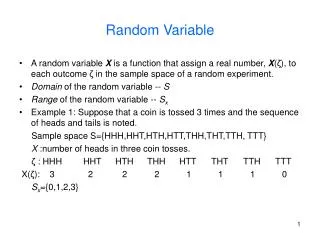
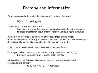
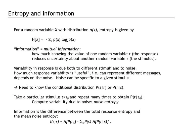
Entropy and information. For a random variable X with distribution p(x), entropy is given by H[ X ] = - S x p( x ) log 2 p( x ) “Information” = mutual information : how much knowing the value of one random variable r (the response)

E N D
Entropy and information For a random variable X with distribution p(x), entropy is given by H[X] = - Sx p(x) log2p(x) “Information” = mutual information: how much knowing the value of one random variable r (the response) reduces uncertainty about another random variable s (the stimulus). Variability in response is due both to different stimuli and to noise. How much response variability is “useful”, i.e. can represent different messages, depends on the noise. Noise can be specific to a given stimulus. Need to know the conditional distribution P(s|r) or P(r|s). Take a particular stimulus s=s0 and repeat many times to obtain P(r|s0). Compute variability due to noise: noise entropy Information is the difference between the total response entropy and the mean noise entropy: I(s;r) = H[P(r)] – Ss P(s) H[P(r|s)] .
Entropy and information Information is symmetric in r and s Examples: response is unrelated to stimulus: p[r|s] = p[r] response is perfectly predicted by stimulus: p[r|s] = d(r-rs)
Maximising information Binary distribution: Entropy Information
Information in single cells: the direct method How can one compute the entropy and information of spike trains? Discretize the spike train into binary words w with letter size Dt, length T. This takes into account correlations between spikes on timescales TDt. Compute pi = p(wi), then the naïve entropy is Strong et al., 1997; Panzeri et al.
Information in single cells: the direct method Many information calculations are limited by sampling: hard to determine P(w) and P(w|s) Systematic bias from undersampling. Correction for finite size effects: Strong et al., 1997
Information in single cells: the direct method Information is the difference between the variability driven by stimuli and that due to noise. Take a stimulus sequence s and repeat many times. For each time in the repeated stimulus, get a set of words P(w|s(t)). Should average over all s with weight P(s); instead, average over time: Hnoise = < H[P(w|si)] >i. Choose length of repeated sequence long enough to sample the noise entropy adequately. Finally, do as a function of word length T and extrapolate to infinite T. Reinagel and Reid, ‘00
Information in single cells Fly H1: obtain information rate of ~80 bits/sec or 1-2 bits/spike.
Information in single cells Another example: temporal coding in the LGN (Reinagel and Reid ‘00)
Information in single cells Apply the same procedure: collect word distributions for a random, then repeated stimulus.
Information in single cells Use this to quantify how precise the code is, and over what timescales correlations are important.
Information in single spikes How much information does a single spike convey about the stimulus? Key idea: the information that a spike gives about the stimulus is the reduction in entropy between the distribution of spike times not knowing the stimulus, and the distribution of times knowing the stimulus. The response to an (arbitrary) stimulus sequence s is r(t). Without knowing that the stimulus was s, the probability of observing a spike in a given bin is proportional to , the mean rate, and the size of the bin. Consider a bin Dt small enough that it can only contain a single spike. Then in the bin at time t,
Now compute the entropy difference: prior conditional and using Assuming , In terms of information per spike (divide by ): Information in single spikes , Note substitution of a time average for an average over the r ensemble.
Information in single spikes Given • note that: • It doesn’t depend explicitly on the stimulus • The rate r does not have to mean rate of spikes; rate of any event. • Information is limited by spike precision, which blurs r(t), • and the mean spike rate. Compute as a function of Dt: Undersampled for small bins
Synergy and redundancy How important is information in multispike patterns? The information in any given event can be computed as: Define the synergy, the information gained from the joint symbol: or equivalently, Negative synergy is called redundancy. Brenner et al., ’00.
Multispike patterns In the identified neuron H1, compute information in a spike pair, separated by an interval dt: Brenner et al., ’00.
Using information to evaluate neural models We can use the information about the stimulus to evaluate our reduced dimensionality models.
Using information to evaluate neural models Information in timing of 1 spike: By definition
Using information to evaluate neural models Given: By definition Bayes’ rule
So the information in the K-dimensional model is evaluated using the distribution of projections: Using information to evaluate neural models Given: By definition Bayes’ rule Dimensionality reduction
Using information to evaluate neural models Here we used information to evaluate reduced models of the Hodgkin-Huxley neuron. Twist model 2D: two covariance modes 1D: STA only
Adaptive coding • Just about every neuron adapts. Why? • To stop the brain from pooping out • To make better use of a limited • dynamic range. • To stop reporting already known facts • All reasonable ideas. • What does that mean for coding? • What part of the signal is the brain meant • to read? • Adaptation can be mechanism for early • sensory systems to make use of statistical • Information about the environment. • How can the brain interpret an adaptive • code? From The Basis of Sensation, Adrian (1929)
Adaptation to stimulus statistics: efficient coding Rate, or spike frequency adaptation is a classic form of adaptation. Let’s go back to the picture of neural computation we discussed before: Can adapt both: the system’s filters the input/output relation (threshold function) Both are observed, and in both cases, the observed adaptations can be thought of as increasing information transmission through the system. Information maximization as a principle of adaptive coding: For optimum information transmission, coding strategy should adjust to the statistics of the inputs. To compute the best strategy, have to impose constraints (Stemmler&Koch) e.g. the variance of the output, or the maximum firing rate.
Adaptation of the input/output relation If we constrain the maximum, the solution for the distribution of output symbols is P(r) = constant = a. Take the output to be a nonlinear transformation on the input: r = g(s). From Fly LMC cells. Measured contrast in natural scenes. Laughlin ’81.
Smirnakis et al., ‘97 Dynamical adaptive coding But is all adaptation to statistics on an evolutionary scale? The world is highly fluctuating. Light intensities vary by 1010 over a day. Expect adaptation to statistics to happen dynamically, in real time. Retina: observe adaptation to variance, or contrast, over 10s of seconds. Surprisingly slow: contrast gain control effects after 100s of milliseconds. Also observed adaptation to spatial scale on a similar timescale.
Dynamical adaptive coding The H1 neuron of the fly visual system. Rescales input/output relation with steady state stimulus statistics. Brenner et al., ‘00
Dynamical adaptive coding As we have seen already, extract the spike-triggered average
Dynamical adaptive coding Compute the input/output relations, as we described before: s = stim . STA; P(spike|s) = rave P(stim|s) / P(s) Do it at different times in variance modulation cycle. Find ongoing normalisation with respect to stimulus standard deviation
Dynamical adaptive coding: naturalistic stimuli Take a more complex stimulus: randomly modulated white noise. Not unlike natural stimuli (Ruderman and Bialek ’97)
Dynamical adaptive coding Find continuous rescaling to variance envelope.
Dynamical information maximization This should imply that information transmission is being maximized. We can compute the information directly and observe the timescale. How much information is available about the stimulus fluctuations? Return to two-state switching experiment. Method: Present n different white noise sequences, randomly ordered, throughout the variance modulation. Collect word responses indexed by time with respect to the cycle, P(w(t)). Now divide according to probe identity, and compute It(w;s) = H[P(w(t))] – Si P(si) H[P(w(t)|si)] , P(si) = 1/n; Similarly, one can compute information about the variance: It(w;s) = H[P(w(t))] – Si P(si) H[P(w(t)|si)] , P(si) = ½; Convert to information/spike by dividing at each time by mean # of spikes.
Other fascinating subjects Maximising information transmission through optimal filtering predicting receptive fields Populations: synergy and redundancy in codes involving many neurons multi-information Sparseness: the new efficient coding