Download

1 / 13
130 likes | 289 Vues
CS122 Engineering Computation Lab Lab 3. Bruce Char Department of Computer Science Drexel University Winter 2012. Review of Lab 2 Cycle. Major Lab 2 concepts to remember Use of “while” versus “for” loops – when each is appropriate

E N D
CS122 Engineering Computation LabLab 3 Bruce Char Department of Computer Science Drexel University Winter 2012
Review of Lab 2 Cycle • Major Lab 2 concepts to remember • Use of “while” versus “for” loops – when each is appropriate • “if” statement enables program to choose between execution paths • Troubleshooting / debugging • Review the “purple” error messages to understand nature of error (sometimes clear, other times not) • Syntax errors – check to see where cursor is blinking within the code edit region
Administrative Notes • Please contact your individual instructors with questions and problems • CLC (room 147 UC) will be staffed from Monday through Friday (odd – quiz - weeks) – 9 AM to 5 PM • In order to be eligible for a lab completion session, please see you instructor at the end of the lab period • In order to be eligible for a makeup lab session, you must contact your instructor for permission as soon as you miss your regularly scheduled lab
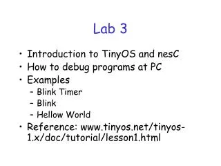
Lab 3 Overview • Based on materials from Chapter 13 and 14 readings • More on user defined functions as represented by Maple proc • We define them and then invoke them to draw things. • We chain functions together to get more complicated drawings. • Using Maple tables to store a collection of data • How to initialize them • How to get a program to enter values into a table • How to use all the values you’ve put into a table in a plot • Multiple assignment • Return multiple proc results as a sequence of variables • Revisit / introduce key plotting concepts • line plots • display feature to enable multiple plots on same grid • Plotting data collected / stored in Maple tables • Plot options – titles, labels, colors
Lab 3 Overview – Part 0 • Part 0.1 – plotting (line and display), proc function • Part 0.2 – introduction to Maple tables and multiple assignments, more on proc usage • Part 0.3 – more on plotting (plot options), procs
Lab 3 Overview – Part 1 • Part 1 – User defined functions that draw things (boxes) • A. - proc to draw rectangular boxes anchored at origin • B. - expand proc from part A. to specify line color and an anchor point other than origin • C. – use of proc developed in B. to draw multiple boxes on same grid • Will be using proc from part B. in Lab 4 as starting point for simulation of a particle bouncing around in a box
Lab 3 Overview – Part 2 • Use a loop and tables to simulate a “time staged” chemical reaction involving 4 chemicals • 2.1 – Calculate the levels of the 4 chemicals as they change over time. Plot the levels of one of the chemicals as it changes over time • Utilizes a proc to encapsulate the simulation code and to pass in the number of time steps as an input parameter • 2.2 – Extend the proc of 2.1 to : • calculate and plot the levels of all 4 chemicals on the same graph • Pass in initial concentration of all 4 reaction components as input parameters • 2.3 – conduct analysis of simulation results from 2.1, 2.2
Lab 3 programming concepts • More about procs • The Maple proc is a user defined function in which: • You can pass parameters into the proc • You can include multiple statements • You can (optionally) return a computed value or series of values • Example • Quadratic := proc(a,b,c) • local x1, x2; • X1 := (-b + sqrt(b^2-4*a*c)) / (2*a); • X2 := (-b - sqrt(b^2-4*a*c)) / (2*a); • return X1, X2; # returns a sequence of numeric results • end proc; • X1solution, X2solution := Quadratic(1, 1, -12); • Note that this example contains a multiple assignment of results
Lab 3 programming concepts • Working with Maple Tables • While a Maple list can hold a series of values, it is not ideal for storing information that is being created dynamically within a loop • Maple tables contain values that all have the same variable name and are differentiated by subscripts • Tables are especially useful in conjunction with loops, where the loop counter variable can be used to represent the subscripts • Working with tables usually requires: • Declaration of the table • Storage of data in the table within a loop • Possible conversion of the table to an equivalent list for use in processes (such as plots) which require lists as input • The example on the next slide illustrates using a table to collect points for subsequent plotting – as in Part 2 of today’s lab
Using Maple Tables to collect data for plotting chemical reaction compositions # Set up initial concentrations A := A0; B := B0; X := X0; Y := Y0; # declare tables indexTab := table(); Atab := table(); for i from 1 to numTimeSteps do newA := A - k1*A*X; … A := newA; indexTab[i] := i; Atab[i] := A; end do: # within Fplot, indexTab and Atab tables are converted to lists display([Fplot(indexTab,Atab,"Green")], title="graph of A", labels=["time", "concentration"]);
Lab 3 programming concepts • A word about time staged simulations • We introduce time staged simulations in the chemical reaction exercise in today’s lab – Part 2 • In a time staged simulation, the loop steps represent time slices • Each iteration of the loop calculates the next generation of values based on correlations using the present generation • In today’s chemical reaction, the concentrations the of 4 reaction components are computed for the next generation (step) from their current values and other coefficients • newA := fn(previousA, B, X, Y) • newB := fn(previousA, B, X, Y) • newX := ………….. • newY := …………..
Lab 3 programming concepts • And finally, some Maple plot features we’ll be using today • Line plotting • Requires with(plottools); • Format line( [x1, y1], [x2, y2] ) • Display multiple plots on same grid • Requires with(plots); • Format display( [line([x1,y1], [x2,y2]) , line([x3,y3],[x4,y4])], color=red); • Plot points contained in X and Y coordinate lists • xList := [1, 2, 3, 4, 5]; • yList := [2, 4, 6, 8, 10]; • Plot(xList, yList, style = point, title=“sometitle”, labels=[“x-axis”, “y-axis”]); • Converting tables to lists (plot commands require Maple lists) • xList := convert(xTab, list); • yList := convert(yTab, list);
Course activities for Quiz week (2/20-2/24) • Quiz 3 will be released on Friday (2/17) at 6 PM • Deadline: Thursday (2/23) at 4:30 PM • Makeup quiz – from Friday (2/24) at 9 AM through Sunday (2/26) at 11:00 PM • 30% penalty • Pre-lab 3 quizlet • From Thursday (2/23 – noon) through Monday (2/27 – 8 AM) • Be sure to visit the CLC for quiz assistance