Download

1 / 27
270 likes | 441 Vues
Selection and Navigation of Mobile Sensor Nodes Using a Sensor Network. Atul Verma, Hemjit Sawant and Jindong Tan Department of Electrical and Computer Engineering Michigan Technological University Houghton, USA Speaker: stephan. Introduction. A hybrid sensor network.

E N D
Selection and Navigation of Mobile Sensor Nodes Using a Sensor Network Atul Verma, Hemjit Sawant and Jindong Tan Department of Electrical and Computer Engineering Michigan Technological University Houghton, USA Speaker: stephan
Introduction • A hybrid sensor network. • Mobile sensor nodes (MSNs) and static sensor nodes can enhance each other’s capability: • MSN can reallocate sensing, networking, and computing resources to provide required coverage and sensing accuracy. • static sensors can guide the MSN to solve some navigation problem.
Modeling of Sensor Network • n: num of static sensor nodes • m: num of mobile sensor nodes • Mobile sensor nodes: • M = { M1, M2, …, Mm} • Configuration of MSN, Mi : • qi (t) = [xi, yi, θi]T • i = 1, 2, ..m • xi, yi: the coordinates of MSN, Mi • θi: the orientation of the MSN with respect to its local coordinate system.
Dynamics of Mi: • ui: the navigational control input • Provide MSN with the direction towards which it should navigate. • Mobile sensor nodes: • S = { S1, S2, …, Sn} • Configuration of static sensor nodes:
Credit Field Based Navigation • A cluster forms • cluster leader: determine whether and how many MSNs are required. • Select • Build up the Navigation Field • Navigation of MSN
Select • find available MSNs using WREQ packet (broadcasted by leader) • MSN reply its weight back to the leader by reversing the route through which the WREQ propagated. • Lower is the weight of the MSN, greater is its probability of navigation of the region of phenomenon.
The navigational controller ui is calculated on the basis of virtual attractive force generated by each static sensor which have the maximum credit field value during each phase of broadcast of navigation packet.
The total energy associated with a MSN is defined: • pij is a vector from MSN, Mi to static sensor nodes Sn in the coordinate frame • || pij || = • ki and kiv are parameters of virtual potential energy and kinetic energy of the MSN.
ui : • Fi is the virtual navigation force generated by static sensor nodes which are at the maximum credit value during each phase of broadcast of navigation packet.
Weight of a Mobile Sensor Node • three metrics to calculate the weight of a MSN: • coverage: leave a smaller coverage hole. • power: saving energy of MSN • distance
coverage : • don’t know the topology of the whole network: • using Voronoi cell approach to determine the coverage of MSN.
Power: • greater the power of MSN, greater is the distance it can traverse and less will be its weight.
Distance: • don’t know the topology of the whole network: • the total num of intermediate nodes through which the WREQ travels is used. • more num of hops more is the weight of MSN.
Weight = Voronoi_cell * distance / power • lower is the weight, more is the probability of MSN reaching the goal.
Simulation • 500 x 500 meters. • Phenom node • Three scenarios: • a uniformly distributed sensor network • a randomly distributed sensor network • a sensor network with a “coverage hole” in it which could represent an “obstacle”.
Dynamic events • Mobile phenom
Conclusion • The algorithm is robust to failures of static sensor. • The algorithms have been verified in an ns-2 environment.