Download
1 / 14
140 likes | 272 Vues
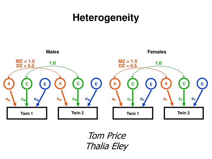
Heterogeneity. Males. Females. MZ = 1.0 DZ = 0.5. MZ = 1.0 DZ = 0.5. 1.0. 1.0. A. A. C. C. A. A. C. E. C. E. E. E. a M. c M. e M. a F. c F. e F. a M. c M. e M. a F. c F. e F. Twin 2. Twin 2. Twin 1. Twin 1. Tom Price Thalia Eley. Males. MZ = 1.0 DZ = 0.5.

E N D
Heterogeneity Males Females MZ = 1.0 DZ = 0.5 MZ = 1.0 DZ = 0.5 1.0 1.0 A A C C A A C E C E E E aM cM eM aF cF eF aM cM eM aF cF eF Twin 2 Twin 2 Twin 1 Twin 1 Tom Price Thalia Eley
Males MZ = 1.0 DZ = 0.5 MZ = 1.0 DZ = 1.0 A C A C E E aM cM eM aM cM eM Twin 1 Twin 2
Females MZ = 1.0 DZ = 0.5 MZ = 1.0 DZ = 1.0 A C A C E E aF cF eF aF cF eF Twin 1 Twin 2
Opposite Sex Pairs a b A C A C E E aM cM eM aF cF eF Male Female
Nested Models A model is said to be ‘nested’ within another model if it estimates the same parameters, but imposes extra constraints on the parameter estimates. Nested models can be compared using the likelihood-ratio test. Each extra constraint gives one more degree of freedom. For example, we may test a series of increasingly parsimonious models by ‘dropping’ (constraining to zero) paths which are likely to be nonsignificant.
Testing For Sex Differences Model Parameters Estimated Full model: aM cM eM aF cF eF aorb Common effects: aM cM eM aF cF eF a = .5,b = 1 Scalar effects: ace k a = .5,b = 1, aM =aF,cM =cF,eM =eF male variance = k x female variance No effects: ace a = .5,b = 1, aM =aF,cM =cF,eM =eF
Practical session In this session we will investigate sex differences in expressive vocabulary in a sample of 2-year-old twins. (The instructors will show you where to find the SPSS dataset.) 1. Using the SPSS script, look at the twin correlations. What do they tell you about possible sex differences? 2. Are there significant mean differences? Regress the mean sex differences from the variables VOCAB1 and VOCAB2. Derive covariance matrices for the residual variables VOCABS1 and VOCABS2. 3. Insert the covariance matrices into the full sex-limited Mx script, and run it. Does the full model fit better than the common effects model? What about the no effects model? 4. If you have time, have a look at the scalar effects script on the handout. How is it different from the full sex-limited model? 5. Think about how these scripts could be modified to test other sources of heterogeneity, such as age or social class.
SPSS script (1) * Compare twin correlations for sex and zygosity groups. USE ALL. SORT CASES BY sexzyg . SPLIT FILE LAYERED BY sexzyg . CORRELATIONS /VARIABLES=vocab1 vocab2 /PRINT=TWOTAIL NOSIG /MISSING=PAIRWISE . * Regress out linear effects of sex and save residuals. SPLIT FILE OFF. REGRESSION /MISSING LISTWISE /STATISTICS COEFF OUTS R ANOVA /CRITERIA=PIN(.05) POUT(.10) /NOORIGIN /DEPENDENT vocab1 /METHOD=ENTER sex1 /SAVE ZRESID (vocabs1). REGRESSION /MISSING LISTWISE /STATISTICS COEFF OUTS R ANOVA /CRITERIA=PIN(.05) POUT(.10) /NOORIGIN /DEPENDENT vocab2 /METHOD=ENTER sex2 /SAVE ZRESID (vocabs2). [continued]
SPSS script (2) * Calculate covariance matrices. USE ALL. COMPUTE filter_$=(atwin = 1 & sexzyg = 1). VALUE LABELS filter_$ 0 'Not Selected' 1 'Selected'. FORMAT filter_$ (f1.0). FILTER BY filter_$. EXECUTE . REGRESSION VARIABLES (COLLECT) /MISSING LISTWISE /DESCRIPTIVES COVARIANCES /DEPENDENT vocabs1 /METHOD=ENTER vocabs2. USE ALL. COMPUTE filter_$=(atwin = 1 & sexzyg = 3). VALUE LABELS filter_$ 0 'Not Selected' 1 'Selected'. FORMAT filter_$ (f1.0). FILTER BY filter_$. EXECUTE . REGRESSION VARIABLES (COLLECT) /MISSING LISTWISE /DESCRIPTIVES COVARIANCES /DEPENDENT vocabs1 /METHOD=ENTER vocabs2. USE ALL. COMPUTE filter_$=(atwin = 1 & sexzyg = 2). VALUE LABELS filter_$ 0 'Not Selected' 1 'Selected'. FORMAT filter_$ (f1.0). FILTER BY filter_$. EXECUTE . [continued]
SPSS script (3) REGRESSION VARIABLES (COLLECT) /MISSING LISTWISE /DESCRIPTIVES COVARIANCES /DEPENDENT vocabs1 /METHOD=ENTER vocabs2. USE ALL. COMPUTE filter_$=(atwin = 1 & sexzyg = 4). VALUE LABELS filter_$ 0 'Not Selected' 1 'Selected'. FORMAT filter_$ (f1.0). FILTER BY filter_$. EXECUTE . REGRESSION VARIABLES (COLLECT) /MISSING LISTWISE /DESCRIPTIVES COVARIANCES /DEPENDENT vocabs1 /METHOD=ENTER vocabs2. USE ALL. COMPUTE filter_$=(sex1 = 1 and sexzyg = 5). VALUE LABELS filter_$ 0 'Not Selected' 1 'Selected'. FORMAT filter_$ (f1.0). FILTER BY filter_$. EXECUTE . REGRESSION VARIABLES (COLLECT) /MISSING LISTWISE /DESCRIPTIVES COVARIANCES /DEPENDENT vocabs1 /METHOD=ENTER vocabs2.
Full sex-limited Mx script (1) ! Genetic correlated factors model ! Full sex-limited model ! use sex-regressed scores in covariance matrices #Define nvar= 1 G1: Male model parameters Data Calc NGroups=9 Begin Matrices; X Lower nvar nvar Free ! G parameters Y Lower nvar nvar Free ! SE parameters Z Lower nvar nvar Free ! NE parameters L Diag nvar nvar Free ! SDs of measures H Diag 1 1 ! scalar .5 O Zero nvar nvar End Matrices; Begin Algebra; A= X * X' ; C= Y * Y' ; E= Z * Z' ; F= A + C + E; End Algebra; Bound -1 1 X 1 1 - X nvar nvar Bound -1 1 Y 1 1 - Y nvar nvar Bound -1 1 Z 1 1 - Z nvar nvarStart .5 All Start 1 L 1 1 - L nvar nvar Matrix H .5 End G2: Female model parameters Data Calc Begin Matrices; X Lower nvar nvar Free ! G parameters Y Lower nvar nvar Free ! SE parameters Z Lower nvar nvar Free ! NE parameters L Diag nvar nvar Free ! SDs of measures H Diag 1 1 ! scalar .5 O Zero nvar nvar End Matrices; Begin Algebra; A= X * X' ; C= Y * Y' ; E= Z * Z' ; F= A + C + E; End Algebra; Bound -1 1 X 1 1 - X nvar nvar Bound -1 1 Y 1 1 - Y nvar nvar Bound -1 1 Z 1 1 - Z nvar nvar Start 1 L 1 1 - L nvar nvar Matrix H .5 End [continued]
Full sex-limited Mx script (2) G5: DZM twin pairs Data NInput_vars= 2 NObservations= XXX Cmatrix Full XXX XXX XXX XXX Cmatrix Full Labels VOCABS1 VOCABS2 Matrices= Group 1 Covariances ( L | O _ O | L ) & ( A + C + E | H@A + C _ H@A + C | A + C + E ) / Option RSidual End G6: DZF twin pairs Data NInput_vars= 2 NObservations= XXX Cmatrix Full XXX XXX XXX XXX Cmatrix Full Labels VOCABS1 VOCABS2 Matrices= Group 2 Covariances ( L | O _ O | L ) & ( A + C + E | H@A + C _ H@A + C | A + C + E ) / Option RSidual End [continued] G3: MZM twin pairs Data NInput_vars= 2 NObservations= XXX Cmatrix Full XXX XXX XXX XXX Labels VOCABS1 VOCABS2 Matrices= Group 1 Covariances ( L | O _ O | L ) & ( A + C + E | A + C _ A + C | A + C + E ) / Option RSidual End G4: MZF twin pairs Data NInput_vars= 2 NObservations= XXX Cmatrix Full XXX XXX XXX XXX Cmatrix Full Labels VOCABS1 VOCABS2 Matrices= Group 2 Covariances ( L | O _ O | L ) & ( A + C + E | A + C _ A + C | A + C + E ) / Option RSidual End
Full sex-limited Mx script (3) G7: DZO twin pairs Data NInput_vars= 2 NObservations= XXX Cmatrix Full XXX XXX Labels VOCABS1 VOCABS2 Begin Matrices; X Lower nvar nvar =X1 Y Lower nvar nvar =Y1 Z Lower nvar nvar =Z1 L Diag nvar nvar =L1 A Lower nvar nvar =X2 C Lower nvar nvar =Y2 E Lower nvar nvar =Z2 M Diag nvar nvar =L2 J Diag nvar nvar Free ! Genetic correlation between males and females K Diag nvar nvar ! Shared environment correlation between males and ! females; can free *either* J *or* K, *not* both O Zero nvar nvar Covariances ( L | O _ O | M ) & ( ( X * X' ) + ( Y * Y' ) + ( Z * Z' ) | ( X * J * A' ) + ( Y * K * C' ) _ ( A * J * X' ) + ( C * K * Y' ) | ( A * A' ) + ( C * C' ) + ( E * E' ) ) / ! NB use covariance matrix with male as 1st twin, ! female as 2nd twin Value .5 J 1 1 - J nvar nvar Value 1 K 1 1 - K nvar nvar Bound -.5 .5 J 1 1 - J nvar nvar Bound -1 1 K 1 1 - K nvar nvar Option RSidual End [continued]
Full sex-limited Mx script (4) G8: Standardise Estimates for Males Data Constraint Matrices = Group 1 I Iden nvar nvar End Matrices; Begin Algebra; U = \sqrt( I . A )~ * A * \sqrt( I . A )~; ! Genetic correlations V = \sqrt( I . C )~ * C * \sqrt( I . C )~; ! Shared environment correlations W = \sqrt( I . E )~ * E * \sqrt( I . E )~; ! Nonshared environment correlations End Algebra; Constrain \d2v( F ) = \d2v( I ); Intervals @95 A 1 1 1 C 1 1 1 E 1 1 1 End G9: Standardise Estimates for Females Data Constraint Matrices = Group 2 I Iden nvar nvar End Matrices; Begin Algebra; U = \sqrt( I . A )~ * A * \sqrt( I . A )~; ! Genetic correlations V = \sqrt( I . C )~ * C * \sqrt( I . C )~; ! Shared environment correlations W = \sqrt( I . E )~ * E * \sqrt( I . E )~; ! Nonshared environment correlations End Algebra; Constrain \d2v( F ) = \d2v( I ); Intervals @95 A 2 1 1 C 2 1 1 E 2 1 1 Intervals @95 J 7 1 1 Options Multiple End ! fix genetic correlations for DZO pairs to .5 ! this tests the common effects model Fix J 7 1 1 - J 7 nvar nvar Value .5 J 7 1 1 - J 7 nvar nvar End ! equate parameters for males and females ! this tests the no effects model Equate X 1 1 1 X 2 1 1 Equate Y 1 1 1 Y 2 1 1 Equate Z 1 1 1 Z 2 1 1 End