Download

1 / 27
270 likes | 577 Vues
An Introduction to Regression with Binary Dependent Variables. Brian Goff Department of Economics Western Kentucky University. Introduction and Description. Examples of binary regression Features of linear probability models Why use logistic regression? Interpreting coefficients

E N D
An Introduction to Regression with Binary Dependent Variables Brian Goff Department of Economics Western Kentucky University
Introduction and Description • Examples of binary regression • Features of linear probability models • Why use logistic regression? • Interpreting coefficients • Evaluating the performance of the model
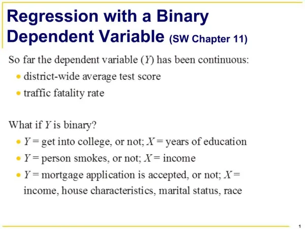
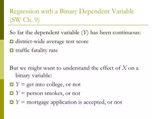
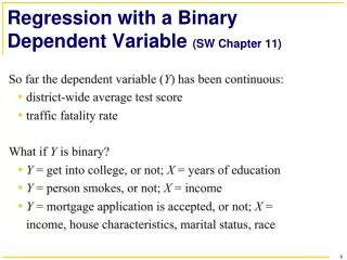
Binary Dependent Variables In many regression settings, the Y variable is (0,1) A Few Examples: • Consumer chooses brand (1) or not (0); • A quality defect occurs (1) or not (0); • A person is hired (1) or not (0); • Evacuate home during hurricane (1) or not (0); • Other Examples?
Scatterplot of with Y=(0,1): Y = Hired-Not Hired; X= Experience Y 1 X 0
The Linear Probability Model (LPM) If we estimate the slope using OLS regression: Hired = α + *Income + e ; • The result is called a “Linear Probability Model” • The predicted values are probabilities that Y equals 1; • The equation is linear – the slope is constant
Picture of LPM Y 1 LPM Regression Line (slope coefficient) Points on regression line represent predicted probabilities For Y for each value of X X 0
An Example: Loan Approvals Data: Dependent Variable: Loaned 1 if Loan Approved, 0 if not Approved by Bank Z Independent Variables ROA = net income as % of total assets of applicant; Debt = debt as % of total assets of applicant; Officer = 1 if loan handled by loan officer A and 0 if handled by officer B;
LPM Results Coefficient on NITA implies 1% increase in ROA increases Probability of loan by 2.2% (0.022)
LPM Weaknesses • The predicted probabilities can be greater than 1 or less than 0 • Probabilities, by definition, have max =1; min = 0; • This is not a big issue if they are very close to 0 and 1 • The error terms vary based on size of X-variable (“heteroskedastic”) – • There may be models that have lower variance – more “efficient” • The errors are not normally distributed because Y takes on only two values • Creates problems for • More of an issue for statistical theorists
Predicted Probabilities in LPM Loans Model In loan case, all of the predicted probabilities fall within (0,1) range
(Binary) Logistic Regression or “Logit” • Selects regression coefficient to force predicted values for Y to be between (0,1) • Produces S-shaped regression predictions rather than straight line • Selects these coefficient through “Maximum Likelihood” estimation technique
Picture of Logistic Regression Y 1 Logistic Regression (non-linear slope coefficient) Points on regression line represent predicted probabilities For Y for each value of X X 0
LPM & Logit Regressions • LPM & Logit Regressions in some cases provide similar answers • If few “outlying” X-values on upper or lower ends then LPM model often produces predicted values within (0,1) band • In such cases, the non-linear sections of the Logit regression are not needed • In such cases, simplicity of LPM may be reason for use • See following slide for an illustration
Logit Model Example where LPM & Logit Results Similar Y LP Model 1 X 0
LPM & Logit: Loan Case • In Loan example the results are similar: • R-square = 98% for regression of LPM-predicted probabilities & Logit-predicted probabilities • Descriptive statistics for both probabilities appear below: • The main difference is the LPM is max/min closer to 0 and 1
SPSS Logistic Regression Output for Loan Approval: Note: The, instead of t-statistics, “Wald” statistics are used to test whether the Coefficients differ from zero; the associated p-values (Sig) have the same Interpretation as in any other regression output
Interpreting Logistic Regression (Logit) Coefficients • The slope coefficient from a logistic regression () = the rate of change in the "log odds" of the event under study as X changes one unit • What in the world does that mean? • We want to know the change in the probability of the event as X changes • In Logistic Regression, this value changes as X-changes (S-shape instead of linear)
Loan Example:Effect of NITA on Probability of LoanNITA coefficient (B) = 0.11
Meaning? • At moderate probabilities (around 0.5) of getting a loan (corresponds to average NITA of about 5), the likelihood of getting a loan increases by 2.75% for each 1% increase in NITA • This estimate is very close to the LPM estimate of 2.2% • At the lower and upper extremes (NITA values -/+ teens), the probability changes by only about 0.9% for a 1 unit increase in NITA
Alternative Methods of Evaluating Logit Regressions Statistics for comparing alternative logit models: • Model Chi-Square • Percent Correct Predictions • Pseudo-R2
Chi-Square Test for Fit • The Chi-Square statistic and associated p-value (Sig.) tests whether the model coefficients as a group equal zero • Larger Chi-squares and smaller p-values indicate greater confidence in rejected the null hypothesis of no
Percent Correct Predictions • The "Percent Correct Predictions" statistic assumes that if the estimated p is greater than or equal to .5 then the event is expected to occur and not occur otherwise. • By assigning these probabilities 0s and 1s and comparing these to the actual 0s and 1s, the % correct Yes, % correct No, and overall % correct scores are calculated. • Note: subgroups for the % correctly predicted is also important, especially if most of the data are 0s or 1s
Percent Correct Results 35% of loan rejected cases (0) were correctly predicted 75% of all cases (0,1) were correctly predicted 94% of loan accepted cases (1) were correctly predicted Note: The model is much better at predicting loan acceptance than loan rejection – this may serve as a basis for thinking about additional variables to improve the model
R2 Problems Y 1 X 0 Notice that whether using LPM or logit, the predicted values on the regression lines are not near The actual observations (which are all either 0 or 1). This makes the typical R-square statistic of no value in assessing how well the model “fits” the data
Pseudo-R2 Values • There are psuedo-R2 statistics that make adjustment for the (0,1) nature of the actual data: two are listed above • Their computation is somewhat complicated but yield measures that vary between 0 and (somewhat close to) 1 much like the R2 in a LP model.
Appendix: Calculating Effect of X-variable on Probability of Y • Effect on probability of from 1 unit change in X = ()*(Probability)*(1-Probability) • Probability changes as the value of X changes • To calculate (1-P) for a given X values: • (1-P) = 1/exp[α + 1*X1 + 2*X2 …] • With multiple X-variables it is common to focus on one at a time and use average values for all but one