Download
1 / 21
210 likes | 431 Vues
Tensors and Component Analysis. Musawir Ali. Tensor: Generalization of an n-dimensional array. Vector: order-1 tensor. Order-3 tensor. Matrix: order-2 tensor. Reshaping Tensors. Matrix to vector. “Vectorizing” a matrix. =. Reshaping Tensors. z. Order-3 tensor to matrix.

E N D
Tensors and Component Analysis Musawir Ali
Tensor: Generalization of an n-dimensional array Vector: order-1 tensor Order-3 tensor Matrix: order-2 tensor
Reshaping Tensors Matrix to vector “Vectorizing” a matrix =
Reshaping Tensors z Order-3 tensor to matrix “Flattening” an order-3 tensor x y A A(1) 1,1,1 1,1,2 1,2,1 1,2,2 2,1,1 2,1,2 2,2,1 2,2,2 1,1,1 2,1,1 1,1,2 2,1,2 1,1,1 1,2,1 2,1,1 2,2,1 1,2,1 2,2,1 1,2,2 2,2,2 1,1,2 1,2,2 2,1,2 2,2,2 A(2) A(3)
n-Mode Multiplication Multiplying Matrices and order-3 tensors A xn M = M A(n) Multiplying a tensor Awith matrix M Ais flattened over dimension n (permute dimensions so that the dimension n is along the columns, and then flatten), and then regular matrix multiplication of matrix M and flattened tensor A(n) is performed
Singular Value Decomposition (SVD) SVD of a Matrix = * * M = U S VT U and V are orthogonal matrices, and S is a diagonal matrix consisting of singular values.
Singular Value Decomposition (SVD) SVD of a Matrix: observations M = U S VT Multiply both sides by MT Multiplying on the left Multiplying on the right MTM = (U S VT)T U S VT MTM = (V S UT) U S VT UTU = I MTM = V S2 VT MMT = U S VT (U S VT)T MMT = U S VT (V S UT) VTV = I MMT = U S2 UT
Singular Value Decomposition (SVD) SVD of a Matrix: observations MMT = U S2 UT MTM = V S2 VT diagonalizations Diagonalization of a Matrix: (finding eigenvalues) • A = W Λ WT • where: • A is a square, symmetric matrix • Columns of W are eigenvectors of A • Λ is a diagonal matrix containing the eigenvalues Therefore, if we know U (or V) and S, we basically have found out the eigenvectors and eigenvalues of MMT (or MTM) !
Principal Component Analysis (PCA) What is PCA? • Analysis of n-dimensional data • Observes correspondence between different dimensions • Determines principal dimensions along which the variance of the data is high Why PCA? • Determines a (lower dimensional) basis to represent the data • Useful compression mechanism • Useful for decreasing dimensionality of high dimensional data
Principal Component Analysis (PCA) Steps in PCA: #1 Calculate Adjusted Data Set Adjusted Data Set: A Data Set: D Mean values: M Mi is calculated by taking the mean of the values in dimension i n dims - … … = data samples
Principal Component Analysis (PCA) Steps in PCA: #2 Calculate Co-variance matrix, C, from Adjusted Data Set, A Co-variance Matrix: C n Note: Since the means of the dimensions in the adjusted data set, A, are 0, the covariance matrix can simply be written as: C = (A AT) / (n-1) n Cij = cov(i,j)
Principal Component Analysis (PCA) Steps in PCA: #3 Calculate eigenvectors and eigenvalues of C Matrix E Matrix E Eigenvalues Eigenvalues x x Eigenvectors Eigenvectors If some eigenvalues are 0 or very small, we can essentially discard those eigenvalues and the corresponding eigenvectors, hence reducing the dimensionality of the new basis.
Principal Component Analysis (PCA) Steps in PCA: #4 Transforming data set to the new basis • F = ETA • where: • F is the transformed data set • ET is the transpose of the E matrix containing the eigenvectors • A is the adjusted data set Note that the dimensions of the new dataset, F, are less than the data set A To recover A from F: (ET)-1F = (ET)-1ETA (ET)TF = A EF = A * E is orthogonal, therefore E-1 = ET
PCA using SVD Recall: In PCA we basically try to find eigenvalues and eigenvectors of the covariance matrix, C. We showed that C = (AAT) / (n-1), and thus finding the eigenvalues and eigenvectors of C is the same as finding the eigenvalues and eigenvectors of AAT Recall: In SVD, we decomposed a matrix A as follows: A = U S VT and we showed that: AAT = U S2 UT where the columns of U contain the eigenvectors of AAT and the eigenvalues of AAT are the squares of the singular values in S Thus SVD gives us the eigenvectors and eigenvalues that we need for PCA
N-Mode SVD • Generalization of SVD Order-2 SVD: Written in terms of mode-n product: By definition of mode-n multiplication: Note: ST = S since S is a diagonal matrix Note: D = S x1 U x2 V = S x2 V x1 U D = U S VT D = S x1 U x2 V D = U ( V S(2) )(1) D = U ( V S )T D = U ST VT D = U S VT
N-Mode SVD • Generalization of SVD D = Z x1 U1 x2 U2 x3 U3 Order-3 SVD: • Z, the core tensor, is the counterpart of S in Order-2 SVD • U1, U2, and U3 are known as mode matrices • Mode matrix Ui is obtained as follows: • perform Order-2 SVD on D(i), the matrix obtained by flattening the tensor D on the i’th dimension. • Ui is the leftmost (column-space) matrix obtained from the SVD above
PCA on Higher Order Tensors Bidirectional Texture Function (BTF) as a Order-3 Tensor Changing illumination, changing view, and changing texels (position) along respective dimensions of the tensor D = Z x1 Ut x2 Ui x3 Uv
PCA on Higher Order Tensors Performing PCA on a Order-3 Tensor Ut texels PCA view + illumination • The matrix, Ut (shown above), resulting from the PCA, consists of the eigenvectors (eigentextures) along its columns • Retrieving/Rendering image: • Transform data to new basis: • F = UtTA • where A is the data in original basis T = Z x1 Ut Image = T x1 F
TensorTextures A cheaper equivalent of PCA: TensorTextures T = Z x1 Ut T = D x2 UiTx3 UvT PCA: TensorTextures: D = Z x1 Ut x2 Ui x3 Uv D =Uv (Ui ( Ut Z(1))(2))(3) D = (Uv Ui) (Ut Z(1))(2) (Uv Ui)-1 D(2) = Ut Z(1) (UiT UvT) D(3) = Z x1 Ut D x2 UiT x3 UvT = Z x1 Ut Recall:
TensorTextures Advantages of TensorTextures over PCA T = Z x1 Ut PCA: T = D x2 UiTx3 UvT TensorTextures: • Independent compression control of illumination and view in TensorTextures, whereas in PCA, the illumination and view are coupled together and thus change/compression of eigenvectors will effect both parameters. • Images represented using fewer coefficients in TensorTextures. • PCA: ( v * i ) basis vectors, each of size t • TensorTextures: ( v + i ) basis vectors, of size v and I • where v = # of view directions, i = # of illumination conditions, and t = # of texels in each image used in the creation of the tensor
TensorTextures Compression vs PCA compression Notice that PCA has one set of basis vectors where as TensorTextures has two: one for illumination, and one for view. This enables selective compression to a desired level of tolerance of perceptual error