Adaptive Meshes on the Sphere: Cubed-Spheres versus Latitude-Longitude Grids

Adaptive Meshes on the Sphere: Cubed-Spheres versus Latitude-Longitude Grids Christiane JablonowskiUniversity of MichiganDec/8/2006

Acknowledgments • The AMR comparison is based on a joint paper with Amik St-Cyr and collaborators from NCAR, submitted to Monthly Weather Review in November 2006 • The AMR Spectral Element Model was mainly developed by Amik St-Cyr, John Dennis & Steve Thomas (NCAR) • The AMR FV model is documented inJablonowski (2004), Jablonowski et al. (2004, 2006) • Contributors to the AMR FV model areMichael Herzog (GFDL) & Joyce Penner (UM)Robert Oehmke (NCAR) & Quentin Stout (UM)Bram van Leer (UM) & Ken Powell (UM)

Overview • Computational Grids on the Sphere • Adaptive mesh refinement (AMR) techniques • Why are we interested in variable resolutions / multi-scales? • Overview of two AMR shallow water models • Finite volume (FV) model • Spectral element model (SEM) • Results: Static and dynamic adaptations • 2D shallow water experiments • Conclusions and Outlook

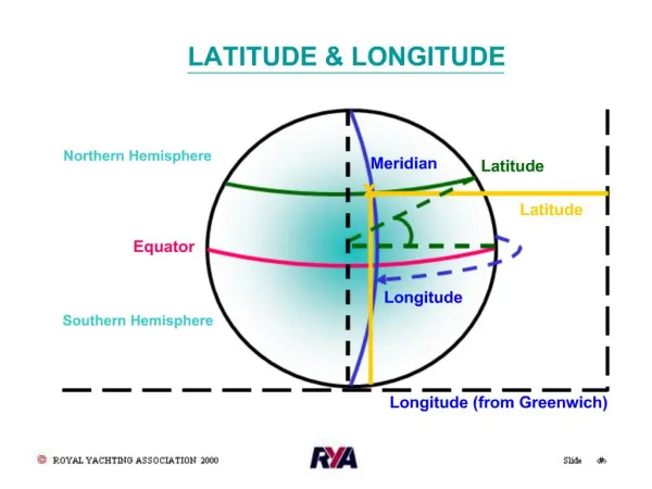
Latitude-Longitude Grid • Popular choice • Meridians converge:polar filters or/andtime steps • Orthogonal

Platonic solids - Regular grid structures • Platonic solids can be enclosed in a sphere

Cubed Sphere Geometry Advection of a cosine bell around the sphere (12 days)at a 45o angle Courtesy of Ram Nair (NCAR)

Adaptive Mesh Refinements (AMR) Cubed-sphere grid:Model SEM Latitude-Longitude grid:Model FV

SEM: Grid Points within Spectral Elements Circles: Gauss-Lobatto-Legendre (GLL) points for vectorsSquares:Gauss-Lobatto (GL) points forscalarsElements are split in case of refinements

FV: Block-Structured Adaptive Mesh Refinement Strategy Self-similar blocks with 3 ghost cells in x & y direction

Other AMR Grids Model ICONIcosahedral grid with nested high-resolution regionsunder development at the German WeatherService (DWD) and MPI, Hamburg Source: DWD

Features of Interest in a Multi-Scale Regime Hurricane Frances Hurricane Ivan September/5/2004

High Resolution: Multi-Scale Interactions 10 km resolution W. Ohfuchi, The Earth Simulator Center, Japan

AMR Transport of a Slotted Cylinder Model FV

Transport of a Slotted Cylinder

Transport of a Slotted Cylinder • Slotted cylinder is reliably detected and tracked

Shallow Water Equations Momentum equation in vector-invariant form Continuity equation vh horizontal velocity vector relative vorticityf Coriolis parameterK= 0.5*(u2 + v2) kinetic energyD horizontal divergence,  damping coefficienth free surface height, hs height of the orographyg gravitational acceleration

Finite Volume (FV) Shallow Water Model • Developed by Lin and Rood (1996), Lin and Rood (1997) • 3D version available (Lin 2004), built upon the SW model: • hydrostatic dynamical core used for climate and weather predictions • Currently part of NCAR’s, NASA’s and GFDL’s General Circulation Models • Numerics: Finite volume approach • conservative and monotonic transport scheme • upwind biased 1D fluxes, operator splitting • van Leer second order scheme for time-averaged numerical fluxes • PPM third order scheme (piecewise parabolic method)for prognostic variables • Staggered grid (Arakawa D-grid) • Orthogonal Latitude-Longitude computational grid

Spectral Element (SEM) Shallow Water Model • Documented in Thomas and Loft (2002), St-Cyr and Thomas (2005), St-Cyr et al. (2006) • 3D version available • Experimental tests within NCAR’s Climate Modeling Software Framework • Numerics: Spectral Elements • Non-conservative and non-monotonic • Allows high-order numerical method • Spectral convergence for smooth flows • GLL and GL collocation points • Non-orthogonal cubed-sphere computational grid

Overview of the AMR comparison • 2D shallow water tests: (Williamson et al., JCP 1992) • Dynamic refinements for pure advection experiments Cosine bell advection test (test case 1) • Static refinements in regions of interest (test case 2) • Dynamic refinements and refinement criteria: Flow over a mountain (test case 5) • Rossby-Haurwitz wave with static refinements (test case 6)

Snapshots: Advection of a Cosine Bell

Error norms: Cosine Bell Advection Days Days Rotation angle = 45:Errors in SEM are lower than in FV

Error norms after 12 days Rotation angle = 0SEM produces undershootsErrors arecomparable

Snapshots: Cosine Bell at day 3 North-polar stereographic projection at day 3 for a = 90 Convergence of blocks in FV

2D Static adaptations FV model: Test case 2,  = 45 • Smooth flow in regimes with strong gradients

Error norms: Test case 2 Days Days Rotation angle = 45:Errors in FV partly due to errors at AMR interfaces

2D Dynamic adaptations in FV Vorticity-basedadaptation criterion 2D shallowwater test #5:15-day run

Snapshots: Flow over a mountain Geopotential height field (test case 5) Longitude Longitude

Snapshots: Flow over a mountain Geopotential height field (test case 5) SEM FV

Error norms: Test case 5 Hours Hours Errors in SEM converge quicker to the NCAR reference solution

Snapshots: Rossby-Haurwitz Wave Geopotential height field (test case 6) at day 7 Smooth flow through static refinement regions

Alternative AMR: Unstructured Triangular Grid Hurricane Floyd (1999) OMEGA model Courtesy ofA. Sarma (SAIC, NC, USA) Colors indicate the wind speed

Conclusions & Outlook • Both grids, cubed-sphere meshes and latitude-longitude grids, are options for AMR techniques • SEM model shows lower error norms in comparison to FV: • Mainly due to high-order numerical method • Partly due to different AMR approach that does not need interpolations of ‘ghost cells’ in blocks • But: SEM is non-monotonic and non-conservative • Cubed-sphere grid has clear advantages: • No convergence of the meridians, no polar filters • But, GLL and GL points for numerical method in SEM are clustered along boundaries of spectral elements • Future interests: Finite-volume AMR method on a cubed-sphere grid

Adaptive Meshes on the Sphere: Cubed-Spheres versus Latitude-Longitude Grids