Download
1 / 16
160 likes | 319 Vues
Methods of Presenting and Interpreting Information. Class 9. Why Use Statistics?. Describe or characterize information Allow researchers to make inferences on samples vis-à-vis the population from which it was drawn Assess validity of hypotheses. Descriptive Measures. Basic Measures

E N D
Why Use Statistics? • Describe or characterize information • Allow researchers to make inferences on samples vis-à-vis the population from which it was drawn • Assess validity of hypotheses
Descriptive Measures • Basic Measures • Central Tendency • Means, median, mode • Supports group comparisons • Variability – whether the Score is Typical • Variability is important because it tells us about whether the distributions of scores across groups are equivalent • Standard deviations is the primary measure (about two thirds of scores tend to fall within one SD of the mean) • Association or correlation – whether variables go together • Positive or negative association • Association tells us what happens to one variable when the other one changes • No causal claim
Hypothesis Testing • Evaluation of the null hypothesis is often stated in terms of the differences in scores between groups. If they are different, we then ask whether the differences were observed by chance (ie, if we repeated the experiment, would we observe the same result? Or a similar result? How often would we observe these differences?) • Types of Error • Type I error – we falsely reject the null hypothesis when in fact it may be true. That is, we assume differences that do not exist. we assume that populations are different when they are alike vis-a-vis the IV-DV relationship • Type I errors are assessed by the level of significance we choose in our statistical tests B if we set significance at .05, we assume that the differences we observed did not happen by more than a 5% chance. That is, we are accepting the odds that the sample differences might have appeared by chance fewer than 5 times in one hundred. The more extreme the criterion, the less likely the sample differences occurred by chance
Type II error – we accept the null hypothesis when, in fact, it is false. That is, we conclude that populations do not differ when in fact they do • Type II errors occur in inverse proportions to Type I errors. That is, we fail to recognize population differences when they may exist. • The only way to reduce Type II error while maintaining a high threshold for Type I error is to use larger sample sizes, or use statistical methods that use more of the available information • Statistical power of a test is the probability that the test will reject the hypothesis tested when a specific alternative hypothesis is true. To calculate the power of a given test, it is necessary to specify β (the probability that the test will lead to the rejection of the hypothesis tested when that hypothesis is true) and to specify a specific alternative hypothesis
Statistical Tests • Choosing a model • Statistical procedures should be keyed to the level of measurement in both the independent and dependent variables • Tests of Association • Chi square -- differences between observed and expected frequencies • Tests of Differences between Means • ANOVA models, ANCOVA models • Tests of differences in distributions (means, std deviations) between groups • Controls for covariates in instances where you assume there may be differences between groups that are systematic (not random)
Multivariate Models • Ordinary Least Squares (OLS) Regression, or Multiple Regression • tells you which combination of variables, and in what priority, influence the distribution of a dependent variable. • It should be used with ratio or interval variables, although there is a controversy regarding its validity when used with ordinal-level variables. • OLS regression is used more often in survey research and non-experimental research, although it can be used to isolate a specific variable whose influence you want to test • You can introduce interaction terms that isolate the effects to specific subgroups (eg, race by gender). • If you do it right, you can control and eliminate statistical correlations between the independent variables • Logistic Regression is a form of regression specifically designed for binary dependent variables (e.g., group membership)
Complex Causation • Structural Equations Models • This family of statistical procedures looks at complex relationships among multiple dependent variables over time. It can accommodate feedback loops, or hypothesized reciprocal relationships. It gives you a probability estimate for each path • Hierarchical Models • When effects are nested – when independent variables exist at more than one ‘level’ of explanation • School research example • School factors (e.g., teacher experience, average SES of parents, computer resources, parent involvement) • Individual factors (e.g., student IQ, family income, parental supervision, number of siblings, sibling school performance)
How Good is the Model? What Does It Tell Us? • Most multivariate models generate probability estimates for each variable in the model, and also for the overall model • Model Statistics: “model fit” or “explained variance” are the two most important • Independent Variables • Coefficient estimate • Standard Error • Statistical Significance
Alternatives to Statistical Significance • Odds Ratio – the odds of having been exposed given the presence of a disease (ratio) compared to the odds of not having been exposed given the presence of the disease (ratio) • Risk Ratio – the risk of a disease in the population given exposure (ratio) compared to the risk of a disease given no exposure (ratio, or the base rate) • Attributable Risk – (Rate of disease among the unexposed – Rate of disease among the exposed) (Rate of disease among the exposed)
In this example, the odds ratio is a way of comparing whether the probability of a certain event is the same for two groups. An odds ratio of 1 implies that the event is equally likely in both groups. An odds ratio greater than one implies that the event is more likely in the first group. An odds ratio less than one implies that the event is less likely in the first group.In the control row, the odds for exclusive breast feeding at discharge are 27 to 20 or odds slightly in favor of exclusive breast feeding. • In the treatment row, the odds are 10 to 32 or odds strongly against exclusive breast feeding. • The odds ratio for exclusive breast feeding at discharge is (27/20) / (10/32) = 4.32. • Since this number is larger than 1, we conclude that breast feeding at discharge is more likely in experimental group.