Download
1 / 37
400 likes | 617 Vues
Theoretical Mechanics - PHY6200. Chapter 6 Introduction to the calculus of variations. Prof. Claude A Pruneau, Physics and Astronomy Department Wayne State University. Introduction. Many mechanics problem more easily analyzed/solved by means of calculus of variation, Lagrange Eqs., etc.

E N D
Theoretical Mechanics - PHY6200 Chapter 6 Introduction to the calculus of variations Prof. Claude A Pruneau, Physics and Astronomy Department Wayne State University
Introduction • Many mechanics problem more easily analyzed/solved by means of calculus of variation, Lagrange Eqs., etc. • We will: • Consider some general principles • Omit formal existence proofs • As an example, consider Fermat’s principle.
air water Fermat’s Principle • Light travels between two points along the path that takes the least amount of time. L
Snell’s Law By construction (geometry): Total travel time: Extremum for : Simplification/Substitution : Snell’s Law :
2 1 Statement of the problem • In classical mechanics, the problem amounts to finding a trajectory between an initial and a final point (boundary conditions). • Express the problem to solve as a minimization problem. • Find a functional that once minimized will yield an optimal trajectory which corresponds to the physical trajectory (according to Newton’s laws of motion).
2 1 Basic Formulation (1 dimension) • Determine a function, y(x), such that the following integral is an extremum. • f(y,y’;x) is a function considered as “given” • Limits of integration are fixed. • y(x), the trajectory is to be varied until an extremum is found for J. • y’(x)=dy(x)/dx • x : independent variable
Basic Formulation (cont’d) • If the optimal trajectory y(x) produces a minimal value for J, then any neighboring trajectory ya(x) corresponds to a large value of J. • Hence by minimizing J, one finds the optimal trajectory. 2 1
Parametric Representation • The function y(x) can be considered with a parametric representation • ya(x) = y(a,x) • Where the variable a denotes a parameter that describes functions close to y(x) but that differ by an “amount” proportional to a. • By definition, a=0 corresponds to the optimal trajectory y(x). • y0(x) = y(0,x)=y(x)
Parametric Representation (cont’d) • Consider the specific representation • y(a,x)=y(0,x)+ (x) • where (x) is some “arbitrary” function of x, with continuous 1st derivative, and vanishing at the boundaries • (x1) = (x2) = 0
Parametric Representation (cont’d) • The functional J is written • This integral has an extremum if • This must be true for all functions h(x) • Note: This is a necessary but not sufficient condition.
Example 1 • Consider the function f(y’;x)=(dy/dx)2. • Where y(x)=x. • Consider h(x)=sin(x) • Find J() between x=0, and x=2. • Show that the stationary value (extremum) of J occurs for =0.
Example 1 - Solution • Let: • y(a,x) = x + sin(x) • Note that by choice/construction, we have • (0) = 0 • (2) = 0 • Proceed to calculate…
Derivation of Euler’s Equation • Calculate the derivative of J • For fixed integration limits, one can change the order of operations
By construction: • Thus:
0 • Integrate 2nd term by parts • The function h(x) being totally arbitrary. • We get • Provided the integrand itself vanishes. • So…
Euler’s Equation This equation yields a solution for y(x) and y’(x) which produces an extremum for J.
Example 2 - Brachistochrone • Consider a particle moving in a constant force field, starting at rest from some point (x1,y1) and ending at (x2,y2). • Find the path (trajectory) that allows the particle to accomplish the motion/transit in the least amount of time.
Example 2 - Solution (1) • Constant force, neglect friction, implies a conservative system. • T+U=constant. • Let U(x=0)=0, and T(0)+U(0)=0. • T=0.5 mv2 • U=-Fx=-mgx y (x1,y1) (x2,y2) x
Example 2 - Solution (2) • Time required for transit:
Example 2 - Solution (3) • Use Euler’s Equation • Thus…
y (0,2pa) (0,pa) (0,0) q (2a,0) cycloid x Example 2 - Brachistochrone - Answer Solution passes through (0,0)
2nd Form of Euler’s Equation • For a function “f” that does not explicitly depend on “x”. 1) 2)
2nd Form of Euler’s Equation (cont’d) • We find: 2nd Form of Euler’s Equation is thus If f does not depend on “x”, there is a conserved quantity
Function with Several Dependent Variables • Consider a more general case where f is a functional of several dependent variables. • E.g. Motion of one particle in 3 dimensions, or many particles…
Several Dependent Variables… • Repeat our previous reasoning… yi(a,x)=yi (0,x)+ ahi(x)
Several Dependent Variables… • So we have • Functions hi are all independent. • Each term of the sum must be null for the above derivative to vanish at a=0. Euler’s Equations for many dependent variables
Euler Equations with Auxiliary Conditions • In many problems, additional constrains come into play. • Consider e.g. motion constrained to a spherical shell, or some other type of curved surface. • Then obviously the path (motion) must be on the surface, and thereby satisfy the equation of the surface, which can be generally be written: g{yi;x}=0 • One therefore introduce constraint equations.
and are thus no longer independent. The variations Euler Equations with Auxiliary Conditions Consider a case: Also include constraints:
No terms in x appear since We write: The constraints equation becomes: or:
The left hand side involves only derivatives of f and g with respect to y and y’, whereas the right hand side involves only derivatives of f and g with respect to z and z’. Because y and z are both functions of x, the two sides may be set equal to some function of x, which we note: -l(x). The complete solution requires one finds three functions: y(x), z(x), and l(x). Fortunately, three relations may be used: the above two equations and the constraints Eq.
The function l(x) is known as Lagrange underdetermined multiplier. In general, if there are many external constraints, one has: m equations m+n unknowns n equations Note that the constraints can also be written: Often more “useful” in problem solutions….
The d Notation • To simplify writing in calculus of variations, one uses a shorthand notation. Consider:
The d Notation • Condition of extremum • Swap d and integral: • Note: • So…
The Notation • Do keep in mind that the d notation is only a shorthand expression for a more detailed and precise quantity. • You can visualize the varied path y as a virtual displacement from the actual path consistent with all forces and constraints. It is to be distinguished from dy (differential displacement) by the condition that dt=0 (fixed time)