Download
1 / 26
260 likes | 390 Vues
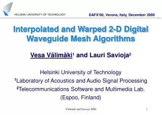
IEEE ICASSP 2001, Salt Lake City, May 2001. INTERPOLATED 3-D DIGITAL WAVEGUIDE MESH WITH FREQUENCY WARPING. Lauri Savioja 1 and Vesa Välimäki 2 Helsinki University of Technology 1 Telecommunications Software and Multimedia Lab. 2 Lab. of Acoustics and Audio Signal Processing

E N D
IEEE ICASSP 2001, Salt Lake City, May 2001 INTERPOLATED 3-D DIGITAL WAVEGUIDE MESH WITH FREQUENCY WARPING Lauri Savioja1 and Vesa Välimäki2 Helsinki University of Technology 1Telecommunications Software and Multimedia Lab. 2Lab. of Acoustics and Audio Signal Processing (Espoo, Finland) http://www.tml.hut.fi/, http://www.acoustics.hut.fi/ Savioja and Välimäki 2001
Outline • Introduction • 3-D Digital Waveguide Mesh • Interpolated 3-D Digital Waveguide Mesh • Optimization of Interpolation Coefficients • Frequency Warping • Simulation Example of A Cube • Conclusions Savioja and Välimäki 2001
Introduction • Digital waveguides are useful in physical modeling of musical instruments and other acoustic systems [8] • 2-D digital waveguide mesh (WGM) for simulation of membranes, drums etc. [2] • 3-D digital waveguide mesh for simulation of acoustic spaces [3] • Numerous potential applications: Acoustic design of concert halls, churches, auditoria, listening rooms, movie theaters, cabins of vehicles, or loudspeaker enclosures Savioja and Välimäki 2001
Former Methods • Ray-tracing • A statistical method • Inaccurate at low frequencies Savioja and Välimäki 2001
Former Methods (2) • Image-source method • Based on mirror images of the sound source(s) • Accurate modeling of low-order reflections • Inaccurate at low frequencies Savioja and Välimäki 2001
New Method • Digital waveguide mesh • Finite-difference method • Sound propagates through the network from node to node • Wide frequency range of good accuracy • Requires much memory Savioja and Välimäki 2001
Sophisticated Waveguide Mesh Structures • In the original WGM, wave propagation speed depends on direction and frequency [3] • Rectangular mesh • More advanced structures improve this problem, e.g., • Triangular and tetrahedral WGMs [3], [7], (Fontana & Rocchesso, 1995, 1998) • Interpolated WGM [5], [6] • Direction-dependence is reduced but frequency-dependence remains ÞDispersion ! Savioja and Välimäki 2001
Interpolated 2-D Waveguide Mesh Hypothetical 8-directional 2-D WGM Interpolated 2-D WGM [5], [6] Original 2-D WGM [2] Savioja and Välimäki 2001
Wave Propagation Speed Interpolated 2-D WGM (bilinear interpolation) Original 2-D WGM 0.2 0.2 0.1 0.1 c c 0 2 0 2 x x -0.1 -0.1 -0.2 -0.2 -0.2 0 0.2 -0.2 0 0.2 c x c x 1 1 Savioja and Välimäki 2001
c 2 x c x 1 Wave Propagation Speed (2) Interpolated 2-D WGM (Optimal interpolation [6]) Original 2-D WGM 0.2 0.1 0 -0.1 -0.2 -0.2 0 0.2 Savioja and Välimäki 2001
Original 3-D Digital Waveguide Mesh • Difference equation for pressure at each node p(n+1, x, y, z) = (1/3) [p(n, x + 1, y, z) + p(n, x – 1, y, z) + p(n, x, y + 1, z) + p(n, x, y – 1, z) + p(n, x, y, z + 1) + p(n, x, y, z – 1)] – p(n–1, x, y, z) where p(n, x, y, z) is the sound pressure at time step n at position (x, y, z) Savioja and Välimäki 2001
Interpolated 3-D Digital Waveguide Mesh • Difference scheme for the interpolated 3-D WGM where coefficients h are Savioja and Välimäki 2001
Interpolated 3-D Digital Waveguide Mesh (2) 2D-diagonal neighbors Original WGM All neighbors in interpolated WGM 3D-diagonal neighbors Savioja and Välimäki 2001
Optimization of Coefficients • Two constraints must be satisfied: 1) 2) Wave travel speed at dc (0 Hz) must be unity • From the first constraint, we may solve 1 coefficient: • Another coefficient can be solved using the 2), for example: Savioja and Välimäki 2001
Optimization of Coefficients (2) • The remaining 2 coefficients can be optimized • We searched for a solution where the difference between the min and max error curves is minimized: ha = 0.124867 h2D = 0.0387600 h3D = 0.0133567 hc = 0.678827 Savioja and Välimäki 2001
Relative Frequency Error (RFE) (a) Original WGM (b) Interpolated WGM Line types Axial — blue 2D-diagonal — cyan 3D-diagonal — red Savioja and Välimäki 2001
Frequency Warping • Dispersion error of the interpolated WGM can be reduced by frequency warping [11] because • Difference between the max and min errors is small • RFE curve is smooth • Postprocessing of the response of the WGM • 3 different approaches: 1) Time-domain warping using a warped-FIR filter [6], [12] 2) Time-domain multiwarping 3) Frequency warping in the frequency domain Savioja and Välimäki 2001
A(z) A(z) A(z) Frequency Warping: Warped-FIR Filter • Chain of first-order allpass filters d(n) s(0) s(1) s(2) s(L-1) sw(n) • s(n) is the signal to be warped • sw(n) is the warped signal • The extent of warping is determined by l Savioja and Välimäki 2001
Frequency Warping: Resampling • Every time-domain frequency-warping operation must be accompanied by a sampling rate conversion • All frequencies are shifted by warping, including those that should not • Resampling factor: (Phase delay of the allpass filter at the zero frequency) • With optimal warping and resampling, the maximal RFE is reduced to 3.8% Savioja and Välimäki 2001
Multiwarping • How to add degrees of freedom to the time-domain frequency-warping to improve the accuracy? • Frequency-warping and sampling-rate-conversion operations can be cascaded • Many parameters to optimize: l1, l2, ... D1, D2,... • We call this multiwarping [12], [13] • Maximal RFE is reduced to 2.0% Savioja and Välimäki 2001
Frequency Warping in the Frequency Domain • Non-uniform resampling of the Fourier transform [14], [15] • Postprocessing of the output signal of the mesh in the frequency domain • Warping function can be the average of the RFEs in 3 different directions • Maximal RFE is reduced to 0.78% Savioja and Välimäki 2001
Improvement of Accuracy Three versions of frequency warping applied to the optimally interpolated WGM (a) Single warping (b) Multiwarping (c) Warping in the frequency domain Savioja and Välimäki 2001
Simulation of a Cubic Space Frequency response of a cubic space simulated using the interpolated WGM (a) Original WGM (b) Interpolated & Multiwarped (c) Interpolated & warped in the frequency domain (red line—analytical) Savioja and Välimäki 2001
Conclusions • Optimally interpolated 3-D digital waveguide mesh • Interpolation yields nearly direction-dependent wave propagation characteristics • Based on the rectangular mesh, which is easy to use • The remaining dispersion can be reduced by using frequency warping • In the time-domain or in the frequency-domain • Future goal: simulation of acoustic spaces using the interpolated 3-D waveguide mesh Savioja and Välimäki 2001
References [1] L. Savioja, T. Rinne, and T. Takala, “Simulation of room acoustics with a 3-D finite difference mesh,” in Proc. Int. Computer Music Conf., Aarhus, Denmark, Sept. 1994. [2] S. Van Duyne and J. O. Smith, “The 2-D digital waveguide mesh,” in Proc. IEEE WASPAA’93, New Paltz, NY, Oct. 1993. [3] S. Van Duyne and J. O. Smith, “The tetrahedral digital waveguide mesh,” in Proc. IEEE WASPAA’95, New Paltz, NY, Oct. 1995. [4] L. Savioja, “Improving the 3-D digital waveguide mesh by interpolation,” in Proc. Nordic Acoustical Meeting, Stockholm, Sweden, Sept. 1998, pp. 265–268. [5] L. Savioja and V. Välimäki, “Improved discrete-time modeling of multi-dimensional wave propagation using the interpolated digital waveguide mesh,” in Proc. IEEE ICASSP’97, Munich, Germany, April 1997. [6] L. Savioja and V. Välimäki, “Reducing the dispersion error in the digital waveguide mesh using interpolation and frequency-warping techniques,” IEEE Trans. Speech and Audio Process., March 2000. [7] S. Van Duyne and J. O. Smith, “The 3D tetrahedral digital waveguide mesh with musical applications,” in Proc. Int. Computer Music Conf., Hong Kong, Aug. 1996. Savioja and Välimäki 2001
[8] J. O. Smith, “Principles of digital waveguide models of musical instruments,” in Applications of Digital Signal Processing to Audio and Acoustics, M. Kahrs and K. Brandenburg, Eds., chapter 10, pp. 417–466. Kluwer Academic, Boston, MA, 1997. [9] J. Strikwerda, Finite Difference Schemes and Partial Differential Equations, Chapman & Hall, New York, NY, 1989. [10] L. Savioja and V. Välimäki, “Reduction of the dispersion error in the triangular digital waveguide mesh using frequency warping,” IEEE Signal Process. Letters, March 1999. [11] A. Oppenheim, D. Johnson, and K. Steiglitz, “Computation of spectra with unequal resolution using the Fast Fourier Transform,” Proc. IEEE, Feb. 1971. [12] V. Välimäki and L. Savioja, “Interpolated and warped 2-D digital waveguide mesh algorithms,” in Proc. DAFX-00, Verona, Italy, Dec. 2000. [13] L. Savioja and V. Välimäki, “Multiwarping for enhancing the frequency accuracy of digital waveguide mesh simulations,” IEEE Signal Processing Letters, May 2001. [14] J. O. Smith, Techniques for Digital Filter Design and System Identification with Application to the Violin, Ph.D. thesis, Stanford University, June 1983. [15] J.-M. Jot, V. Larcher, and O. Warusfel, “Digital signal processing issues in the context of binaural and transaural stereophony,” in 98th AES Convention, Paris, Feb. 1995. Savioja and Välimäki 2001