Download
1 / 56
560 likes | 810 Vues
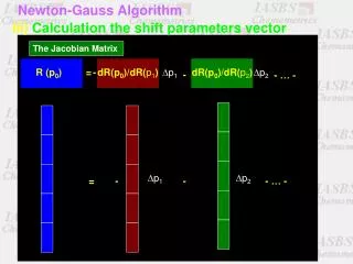
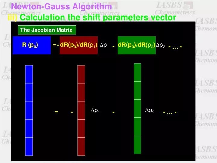
Newton-Gauss Algorithm. =. -. dR(p 0 )/dR( p 1 ). D p 1. dR(p 0 )/dR( p 2 ). D p 2. -. - … -. R (p 0 ). D p 2. -. - … -. iii) Calculation the shift parameters vector. The Jacobian Matrix. D p 1. =. -. Newton-Gauss Algorithm. iii) Calculation the shift parameters vector.

E N D
Newton-Gauss Algorithm = - dR(p0)/dR(p1) Dp1 dR(p0)/dR(p2) Dp2 - - … - R (p0) Dp2 - - … - iii) Calculation the shift parameters vector The Jacobian Matrix Dp1 = -
Newton-Gauss Algorithm iii) Calculation the shift parameters vector The Jacobian Matrix r(p0) Dp J Dp1 Dp2 r(p0) = - J Dp = - Dp = - (JTJ)-1 JT r(p0) Dp = - J+ r(p0)
Newton-Gauss Algorithm R(k1,k2) J(k2) r(k1,k2) Vectorised J(k1) Vectorised J(k2) iii) Calculation the shift parameters vector The Jacobian Matrix J(k1)
Newton-Gauss Algorithm = - Dk1 - Dk2 r(0.3,0.15) = -J(0.3) Dk1 - J(0.15) Dk2 iii) Calculation the shift parameters vector Dp = - J+ r(0.3, 0.15) Dp = [0.0572 0.0695] p = p0 + Dp p = [0.3 0.15] + [0.0572 0.0695] = [0.3572 0.2195] ssq_old = 1.6644 ssq = 0.03346
Newton-Gauss Algorithm ssq old - ssq Abs ( ) ≤ m ssq old iv) Iteration until convergence Convergence Criterion Depending on the data, ssq can be very small or very large. Therefore, a convergence criterion analyzing the relative change in ssq has to be applied. The iterations are stopped once the absolute change is less than a preset value, m, typically m=10-4
Newton-Gauss Algorithm ssq const.? no guess parameters, p=pstart Calculate residuals, r(p) and sum of squares, ssq yes End, display results Calculate Jacobian, J Calculate shift vector Dp, and p = p + Dp
ssq sA = ( )0.5 nt × nl – (np + nc × nl) Error Estimation The availability of estimates for the standard deviations of the fitted parameters is a crucial advantage of the Newton-Gauss algorithm. Hess matrix H = JTJ The inverted Hessian matrix H-1, is the variance-covariance matrix of the fitted parameters. The diagonal elements contain information on the parameter variances and the off-diagonal elements the covariances. si = sA (di,i)0.5
ng function Using Newton-Gauss algorithm for multivariate fitting
r_cons function Introducing the model for consecutive kinetics to ng function
Initial estimates kinfit5 Executing the ng function
? Exactly read the ng.m, r_cons.m and kinfit5.m files and explain them
Rank deficiency and fitting Second order kinetics k A + B C Rank deficiency in concentration profiles [A] + [C] = [A]0 [B] + [C] = [B]0 a [A] - [B] + (a - 1) [C] = 0 [B]0 = a [A]0 Linear dependency [B] + [C] = a [A] + a [C]
[A]0 = 1 [B]0 = 1.5 k = 0.3 A = C E + R E = C \ A
Reconstructed data Measured data Residuals
? Use ng function for determination of pKa of weak acid HA
The Marquardt modification Generally, The Newton-Gauss method converges rapidly, quadratically near the minimum. However, if the initial estimates are poor, the functional approximation by the Taylor series expansion and the linearization of the problem becomes invalid. This can lead to divergence of the ssq and failure of the algorithm. H = JT J Dp = - (H + mp × I)-1 JT r(p0) The Marquardt parameter (mp) is initially set to zero. If divergence of the ssq occurs, then the mp is introduce (given a value of 1) and increased (multiplication by 10 per iteration) until the ssq begins to converge. Increasing the mp shortens the shift vector and direct it to the direction of steepest descent. Once the ssq convergences the magnitude of the mp is reduced (division by 3 per iteration) and eventually set to zero when the break criterion is reached.
Newton-Gauss method and poor estimates of parameters Measured data Considered model: Consecutive kinetic Estimated parameters: k1=4 k2=2 Original parameters: k1=0.4 k2=0.2
Newton-Gauss-Levenberg-Marquardt Algorithm ssqold< = > ssq mp=0 guess parameters, p=pstart initial value for mp Calculate residuals, r(p) and sum of squares, ssq < = yes End, display results no > mp ×10 mp / 3 mp=0 Calculate Jacobian, J Calculate shift vector Dp, and p = p + Dp
nglm.m Newton-Gauss-Levenberg-Marquardt Algorithm for non-linear curve fitting