Download
1 / 38
380 likes | 478 Vues
Details of space charge calculations for J-PARC rings. KEK Portion. JAERI Portion. J-PARC accelerator complex. Phase 1 + Phase 2 = 1,890 Oku Yen (= $1.89 billions if $1 = 100 Yen). Phase 1 = 1,527 Oku Yen (= $1.5 billions) for 7 years. JAERI: 860 Oku Yen (56%), KEK: 667 Oku Yen (44%).

E N D
KEK Portion JAERI Portion J-PARC accelerator complex • Phase 1 + Phase 2 = 1,890 Oku Yen (= $1.89 billions if $1 = 100 Yen). • Phase 1 = 1,527 Oku Yen (= $1.5 billions) for 7 years. • JAERI: 860 Oku Yen (56%), KEK: 667 Oku Yen (44%).
Repetition of 3GeV Synchrotron • injection 500μs • injection turns~350 • particles per pulse8.3e13 • acceleration20 ms • extraction<1μs extraction injection acceleration
Repetition of 50 GeV Synchrotron • injection 0.17s • particles per pulse3.3e14 • acceleration1.96 s • extraction (slow)0.7s extraction acceleration injection
Two approaches • A whole cycle of 3 GeV synchrotron takes 20 ms. • Full simulation with self-consistent model is possible. • Tracking parameters (# of macro particles, grid size, etc) have to be optimized. • Only injection period of 50 GeV synchrotron takes 0.6 s (or a bit less). • Not realistic to make self-consistent simulation. • Frozen space charge model might be justified because of well defined particle distribution.
Examples of full tracking for 3GeV Syn. • Things are included. • Injection painting • Multipole errors • Misalignment • Acceleration • Aperture of all elements • Image in a circular pipe • Things are not included. • Scattering at foil. • RF jitter • Impedance Different colors shows results of different number of macro particles. Results within 3 months (1,000,000~200,000) 3 months (100,000) 5 weeks (50,000) 2 weeks (20,000)
Other tracking parameters Number of azimuthal mode Max. mode = 4, 8, 16 Number of z grids z grids = 10, 20, 30, 40,50
Detailed study results • Correlated and anti-correlated painting • COD and beam loss • Coupled with strong chromaticity correction sextupole, COD introduces nonlinearity of all harmonics. • Beam intensity dependence
Correlated and anti-correlated painting correlated anti-correlated 0.5 s for injection There is particle loss even during injection period.
Phase space density right after injection and at 3 ms later correlated anti-correlated horizontal vertical at 0.5 ms at 0.5 ms at 3 ms at 3 ms
COD and beam loss Coupled with strong chromaticity correction sextupole, COD introduces nonlinearity of all harmonics. rms COD 0 mm 0.2 mm 0.5 mm 1.0 mm
Phase space density for different COD Ver. Hor. rms COD 0 mm 0.2 mm 0.5 mm 1.0 mm rms COD 0 mm 0.2 mm 0.5 mm 1.0 mm • No difference in core density. • Tails are developed with COD.
Beam intensity dependence 20mA 30mA cf. 30mA is design value which deliver 0.6 MW beam from RCS with tune spread of ~0,25.
Intensity dependence 20mA 30mA 20mA 30mA • Core density is reduce with 30 mA. • (lower order resonance is involved?) • Tails are also developed.
Summary of self-consistent simulation • A whole cycle of 3 GeV Syn can be simulated even though it takes a few months. • Horizontal and vertical coupling is the source which makes anti-correlated painting worse. • Increase of particle loss due to larger COD is attributed to tail development. Higher order effects are involved. • Intensity limitation may be explained with lower order resonance. That is a regime where coherence picture is applicable.
Example of beam loss during injection with frozen space charge model • Model assumes • Particle distribution is Gaussian. • Emittance is constant. • dp/p is finite and there are synchrotron oscillations. • Transverse space charge force depends on longitudinal position.
Tracking model • “Frozen model” of space charge is adopted. • Space charge potential is fixed throughout a tracking. • No self-consistency. • No coherent oscillations. • Gaussian charge distribution in 3D is assumed. • Lattice nonlinearities and misalignment errors are included. • Aperture of magnets and collimator are included so that we can estimate beam loss. • Macro particles (1,000) of 3D Gaussian distribution with 2 sigma cut are tracked for 0.12s (original design value for accumulation) or more.
Some numbers • Emittance(2sigma) 54 pi mm-mrad (36pi, 45pi, 64pi) • Acceptance at collimator 71 pi mm-mrad for H and V • Acceptance at magnets > 81 pi mm-mrad • Circulating current 10 A (3.3E14 ppp) • Incoherent tune shift -0.16 • Bare tune (22.42, 20.80)
COD • Chromaticity sextupoles coupled with COD introduce beta modulation and higher harmonics of nonlinearity. • Survival at 0.12s after injection. • COD shows a rms value. Maximum is about 3 times. • Collimator aperture is adjusted taking a local COD into account. • We expect COD(rms) is less than 0.5mm after correction. • The loss is not linear as COD. survival at 0.12s (%) 80 85 90 95 100 0 0.5 1.0 1.5 2.0 COD (rms) (mm)
Different lattices • Although rms COD is almost same, different lattices (seeds) give different results. • Previous example is the worst case among three. survival (%) 96 97 98 99 100 0 0.05 0.1 time (s)
Beam current Blue: COD=0.5mm Red: COD=1.0mm • The pattern of COD is the same for both. Magnitude is different. • The design current is 10A. survival at 0.12s (%) 80 85 90 95 100 0 5.0 10 15 beam current (A)
Initial emittance • Acceptance at collimator is fixed at 71 pi mm-mrad. • Space charge force is fixed according to the initial emittance. • We expect 54 pi mm-mrad emittance shaped at the 3-50BT collimator. • Collimator acceptance should be optimized to have the maximum survival. survival at 0.12s (%) 80 85 90 95 100 30 40 50 60 70 80 initial emittance (pi mm-mrad)
Beam loss at collimator (h=18)total 0.72 MW COD (rms) = Red: 0mm Yellow: 0.2mm Green: 0.5mm All the particles hit collimator first.
Beam loss at collimator (h=18)total 0.58 MW COD (rms) = Red: 0mm Yellow: 0.2mm Green: 0.5mm All the particles hit collimator first.
Frozen model with acceleration phis dp/p bunch length
99% emittance and beam loss Acceleration starts right after injection. Acceleration starts at 0.16 s after injection.
Single particle behavior Timing of hitting collimator • Tracking without aperture limit to see single particle behavior. • Slow growth of amplitude. • Not obvious correlation with synchrotron oscillations. Trapping? horizontal position (m) -0.1 -0.05 0 0.50 0.1 0 0.01 0.02 0.03 0.04 0.05 time (s)
Single particle behavior • Track a single particle which is lost in 0.6 s. • Look at betatron oscillation amplitude and transverse tune as a function of turn until a particle is lost. • For example, there are • 38 lost particles (out of 1000) when rms COD is 0mm. • 40 lost particles (out of 1000) when rms COD is 0.2 mm. • 52 lost particles (out of 1000) when rms COD is 0.5 mm.
#1 #3 #2 H V H V #4 #5 #6 amplitude turn number (~ 10,000 turns) rms COD is 0.5 mm
#7 #8 #9 H V H V #10 #11 #12 amplitude turn number (~ 10,000 turns) rms COD is 0.5 mm
H V #13 #14 #15 • Horizontal amplitude always • increases and gets to the aperture • limit. • Vertical amplitude always decreases. • Coupling between H and V is manifest. H V amplitude #16 rms COD is 0.5 mm turn number (~ 10,000 turns)
In tune space 2nx-ny=24 ny-20 ny-20 bare tune nx-2ny=-19 nx-22 nx-22 Blue points are intermediate tune of lost particles. Red points are tune just before particles are lost. Tune before particle loss are same with and without COD.
Coupling between H and V is manifest, but • Tune space plot does not show resonance driving term. • 2nx-ny=24 is skew and cannot be excited even with finite dp/p and dispersion in a lattice. • If there is any way to reduce a driving term. • Since the source is not identified, it is difficult.
Summary of frozen space charge simulation • Particle loss occurs because horizontal amplitude increases and hits the collimator aperture. The source of the increase is a coupling between H and V. • With finite COD, particle loss occurs with less turns. However, transverse tune when a particle loss occurs does not depend on COD magnitude. • Loss is very slow process: the order of 104 turns. Time scale of horizontal and vertical coupling is also same order.
Basic loop of calculation Advance particle coordinates do ip=1,np (200,000) Simpsons uses Fourier expansion in azimuthal direction. Make parallel processing of Fourier modes. Calculate space charge potential based on particle positions. do imode=1,nmode (16) Apply space charge kicks to all particles do ip=1,np (200,000)
Distribution of workload (4 CPUs) with MPI Add up all E-fields 4 CPU works in the same way imode =0,1,2 imode =3,4,5,6 imode =7~11 imode =12~16