Download
1 / 27
690 likes | 1.73k Vues
Remote Sensing Hyperspectral Remote Sensing. 1. Hyperspectral Remote Sensing. Collects image data in many narrow contiguous spectral bands through the visible and infrared portions of spectrum The band width is < 10nm 1mm = 1,000 m m 1 m m = 1,000nm.

E N D
1. Hyperspectral Remote Sensing • Collects image data in many narrow contiguous spectral bands through the visible and infrared portions of spectrum • The band width is < 10nm 1mm = 1,000mm 1mm= 1,000nm http://en.wikipedia.org/wiki/Hyperspectral_imaging
Vegetation Spectral Reflectance extracted from AVIRIS data http://www.csr.utexas.edu/projects/rs/hrs/hyper.html
1. Hyperspectral ... • Many features on Earth have diagnostic spectral characteristics at a resolution of 20-40nm • Hyperspectral image data can identify these features directly • While the traditional multispectral image data cannot
1. Hyperspectral .. • Acquires a complete reflectance spectrum for each pixel • Improves the identification of features and quantitatively assess their physical and chemical properties • The target of interests includes minerals, water, vegetation, soils, and human-made materials
2. History AIS • Airborne Imaging Spectrometer (AIS) developed in 1982 was the first hyperspectral system • 128 bands, 0.9-2.4mm • Designed to identify minerals
2. History .. AVIRIS • Airborne Visible/Infrared Imaging Spectrometer was developed in 1987 • 224 bands, 0.4-2.5mm, 10nm band width • The first to cover the visible portion of spectrum • Provides a large number of images for research and application
2. History .. • FLI (fluorescence line imager) • ASAS (Advanced Solid-State Array Spectrometer) • CASI (Compact Airborne Spectrographic Imager) • HYDICE (hyperspectral digital image collection experiment) • HyMap (Airborne Hyperspectral Scanners) • in the 1990’s
2. History .. • Earth Observing-1 (EO-1) • The first space borne hyperspectral system was launched in 2000 • Developed by NASA and ESA (European Space Agency)
2. History .. Earth Observing-1 (EO-1) • Three instruments are onboard EO-1 - Hyperon 220 bands, 0.4-2.5mm, 30m spatial resolution
Pearl Harbor http://eo1.gsfc.nasa.gov/miscPages/home.html
3. Applications • The initial motivation is mineral identification • Many minerals have unique diagnostic reflectance characteristics • Plants are composed of the same few compounds and should have similar spectral signatures
3. Applications • The identification of biochemical and biophysical characteristics of plants has been a major application area • Traditional wide-band multispectral images have limited value in studying dominant plant characteristics, such as red absorption, NIR reflectance, and mid infrared absorption
3. Applications .. • Leaf area index and crown closure • Species and composition • Biomass • Chlorophyll • Nutrients, nitrogen, phosphorous, potassium • Leaf and canopy water content
4. Analysis Methods • Methods used to extract biochemical and biophysical characteristics from hyperspectral data
4. Analysis Methods .. Spectral matching • Cross-correlagram spectral matching (CCSM) • Taking into consideration the correlation coefficient between a target spectrum and a reference spectrum
4. Analysis Methods .. Spectral index • Hyperspectral data provide greater chance and flexibility to choose spectral bands • Traditional multispectral data only provide the choice of red and NIR bands • Narrowband vegetation index to assess characteristics of bioparameters, chlorophyll, foliar chemistry, water, and stress
4. Analysis Methods .. Absorption and spectral position • Quantitative assessment of absorption allows for abundance estimation • The method measures the depth of valleys in a spectral curve to assess absorptions • and identifies high points in a spectral curve to assess spectral position of certain features
4. Analysis Methods .. Hyperspectral transformation • Reduces the data dimension • Principle Component Analysis (PCA) to reduce the number of bands • Canonical Discriminant Analysis to determine the relationship between quantitaive variables and nominal classes
4. Analysis Methods .. Spectral unmixing • The number of bands is much greater than the number of endmembers • Statistical methods are used to solve for Fs and Es
Spectral Mixture Analysis .. Linear mixture models - assuming a linear mixture of pure features Endmembers - the pure referenc signatures Weight - the proportion of the area occupied by an endmember Output - fraction image for each endmember showing the fraction occupied by an endmember in a pixel
Spectral Mixture Analysis .. Two basic conditions I. The sum of fractions of all endmembers in a pixel must equal 1 Fi = F1 + F2 + … + Fn = 1 II. The DN of a pixel is the sum of the DNs of endmembers weighted by their area fractions D = F1 D1 + F2 D2 + … + Fn Dn+E
Spectral Mixture Analysis .. One Dequation for each band, plus one Fi equation for all bands Number of endmembers = number of bands + 1: One exact solution without the E term Number of endmembers < number of bands +1: Fs and E can be estimated statistically Number of endmembers > number of bands +1: No unique solution
4. Analysis Methods .. Image classification • Faces difficulties caused by the high dimensionality, the high correlation between bands, and a limited number of training samples • Requires to maximize the ratio of between-class variance and within-class variance of training samples to separate class centers as far as possible
4. Analysis Methods .. Empirical analysis • Most commonly used methods correlate biophysical/biochemical characteristics with spectral reflectance/spectral indices in the visible, NIR, and SWIR wavelengths at leaf, canopy, or community level • Simple methods, such as regression, often have higher accuracy, but cannot be applied directly to other areas