Download
1 / 33
330 likes | 491 Vues
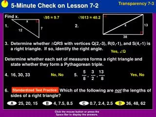
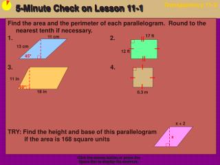
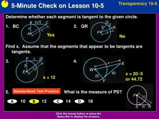
5-Minute Check on Lesson 2-2b. What is the shape of a normality plot if the distribution is approximately normal? Given a normal distribution with = 4 and = 2, Find P(x < 2) P(x > 5) P(1< x < 5) x, if P(x) = 0.95 x, if P(x) = 0.05. linear a line.

E N D
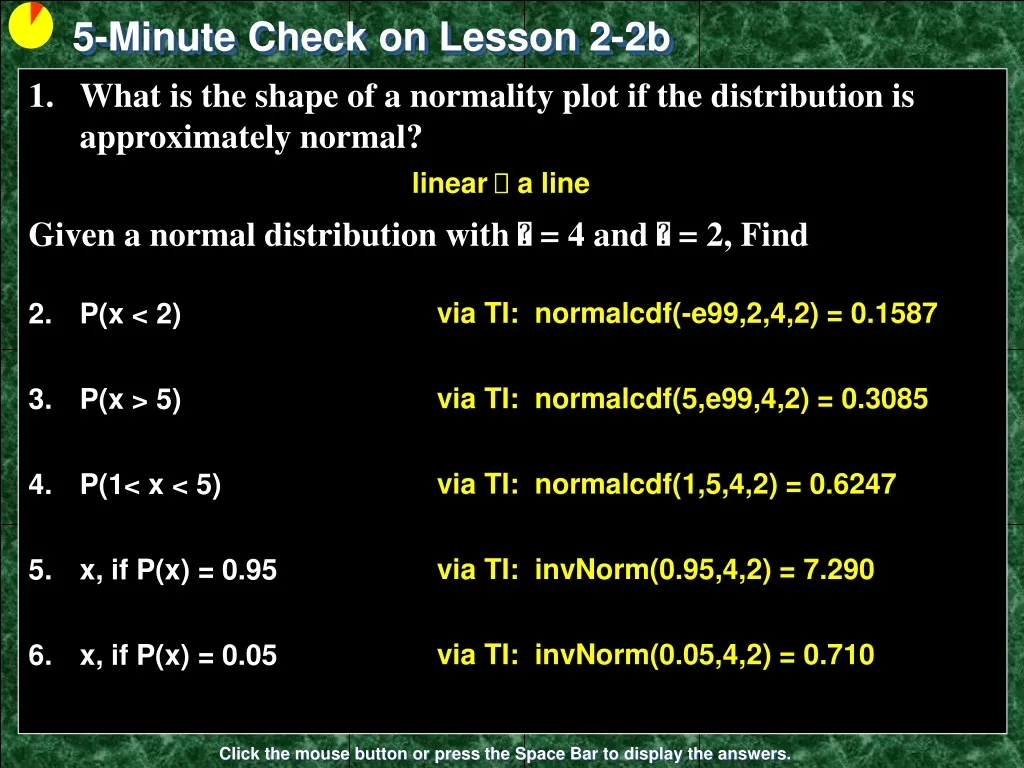
5-Minute Check on Lesson 2-2b What is the shape of a normality plot if the distribution is approximately normal? Given a normal distribution with = 4 and = 2, Find P(x < 2) P(x > 5) P(1< x < 5) x, if P(x) = 0.95 x, if P(x) = 0.05 linear a line via TI: normalcdf(-e99,2,4,2) = 0.1587 via TI: normalcdf(5,e99,4,2) = 0.3085 via TI: normalcdf(1,5,4,2) = 0.6247 via TI: invNorm(0.95,4,2) = 7.290 via TI: invNorm(0.05,4,2) = 0.710 Click the mouse button or press the Space Bar to display the answers.
Lesson 2 - R Review of Chapter 2Describing Location in a Distribution
Objectives • Be able to compute measures of relative standing for individual values in a distribution. This includes standardized values z-scores and percentile ranks. • Use Chebyshev’s Inequality to describe the percentage of values in a distribution within an interval centered at the mean • Demonstrate an understanding of a density curve, including its mean and median
Objectives • Demonstrate an understanding of the Normal distribution and the 68-95-99.7 Rule (Empirical Rule) • Use tables and technology to find • (a) the proportion of values on an interval of the Normal distribution and • (b) a value with a given proportion of observations above or below it • Use a variety of techniques, including construction of a normal probability plot, to assess the Normality of a distribution
Vocabulary • none new
Measures of Relative Standing x – μ Z = ---------- Z ~ N(0, 1) Normal(, ) σ • Z-score: measures the number of standard deviations away from the mean an x value is • Invnorm(percentile[,μ,σ]) gives us the z-value associated with a given percentile • Empirical Rule vs Chebyshev’s Inequality
Density Curves • The area underneath a density curve between two points is the proportion of all observations • Sum of the area underneath density curve is equal to 1 • The median is the equal area point • The mean is the “balance” point • The mean is pulled more toward any skewness
Normal Distribution μ ± 3σ μ ± 2σ μ ± σ 99.7% • Symmetric, mound shaped, distributionmean is and standard deviation is X ~ N (, ) • Empirical Rule (68-95-99.7) applies • Mean is highest point; ± one standard deviation is at the two inflection points (where the curve goes bowl down to bowl up) 95% 68% 2.35% 2.35% 34% 34% 13.5% 13.5% 0.15% 0.15% μ - 2σ μ μ + 2σ μ - 3σ μ - σ μ + σ μ + 3σ
a a a b Obtaining Area under Standard Normal Curve
a a a b Obtaining Area under Any Normal Curve
Assessing Normality • Use calculator to view • Normal probability plots to access the linearity of the graph (linear plot indicates normal distribution) • Histogram and/or boxplot to access the symmetry and mound shape of the distribution • Use Empirical Rule (68-95-99.7) to evaluate how “normal-like” the distribution is
TI-83 Help • normalpdfpdf = Probability Density FunctionThis function returns the probability of a single value of the random variable x. Use this to graph a normal curve. Not used very often. Syntax: normalpdf (x, mean, standard deviation) • normalcdf cdf = Cumulative Distribution FunctionTechnically, it returns the percentage of area under a continuous distribution curve from negative infinity to the x. Syntax: normalcdf (lower bound, upper bound, mean, std dev)(note: lower bound is optional and we can use -E99 for negative infinity and E99 for positive infinity) • invNorminv = Inverse Normal PDFThe inverse normal probability distribution function will find the precise value at a given percent based upon the mean and standard deviation. Syntax: invNorm (probability, mean, std dev)
Uniform Distribution • Rectangular-shaped distribution with all outcomes equally likely; area sums to 1 • Discrete example: one dice1/6 probability of each number • Continuous example: a fire drill equally likely at any time during a periodlength = 50 (minutes) and height = (1/50) P(x=1) = 0 P(x ≤ 1) = 0.33 P(x ≤ 2) = 0.66 P(x ≤ 3) = 1.00 P(x=0) = 0.25 P(x=1) = 0.25 P(x=2) = 0.25 P(x=3) = 0.25
What You Learned Measures of Relative Standing • Find the standardized value (z-score) of an observation. Interpret z-scores in context • Use percentiles to locate individual values within distributions of data • Apply Chebyshev’s inequality to a given distribution of data
What You Learned Density Curves • Know that areas under a density curve represent proportions of all observations and that the total area under a density curve is 1 • Approximately locate the median (equal-areas point) and the mean (balance point) on a density curve • Know that the mean and median both lie at the center of a symmetric density curve and that the mean moves farther toward the long tail of a skewed curve
What You Learned Normal Distribution • Recognize the shape of Normal curves and be able to estimate both the mean and standard deviation from such a curve • Use the 68-95-99.7 rule (Empirical Rule) and symmetry to state what percent of the observations from a Normal distribution fall between two points when the points lie at the mean or one, two, or three standard deviations on either side of the mean
What You Learned Normal Distribution (continued) • Use the standard Normal distribution to calculate the proportion of values in a specified range and to determine a z-score from a percentile • Given a variable with a Normal distribution with mean and standard deviation , use Table A and your calculator to • determine the proportion of values in a specified range • calculate the point having a stated proportion of all values to the left or to the right of it
What You Learned Assessing Normality • Plot a histogram, stemplot, and/or boxplot to determine if a distribution is bell-shaped • Determine the proportion of observations within one, two, and three standard deviations of the mean and compare with the 68-95-99.7 rule (Empirical rule) for Normal distributions • Construct and interpret Normal probability plots
Summary and Homework • Summary • Remember SOCS • Z-score (standard deviations from the mean) • Chebyshev’s inequality vs 68-95-99.7 Rule • Determine proportions of given parameters • Assessing Normality • Empirical Rule • Normality plots • Normal & Standard Normal Curves’ Properties • Homework • pg 162 – 163; problems 2.51 – 2.59
Problem 1 Scores on a test have mean 75 and standard deviation 6. The teacher is considering curving these grades. (a) If the teacher adds 5 points to all individual grades, the class mean will be ___________ and the standard deviation will be _____________. (b) If the teacher increases all grades by 10%, the class mean will be ________________ and the standard deviation will be _________________. 75 + 5 = 80 6 (unchanged) 75 + 7.5 = 82.5 6(1.1) = 6.6
Problem 2 Suppose that the juice dispensers in a school dining hall are filled each morning with 20 gallons of juice. Records show that a probability density function describing the daily juice consumption j is: f(j) = 0.1 – 0.005j if 0 ≤ j ≤ 20 A sketch of this density curve is provided in the space to the right. (a) Verify that f is a valid density function. Area under the curve must be 1! Area of triangle = ½ b h = ½ (20) (0.1) = ½ (2) = 1 Yes it is a valid density function
Problem 3 Scores on an intelligence test are normally distributed with mean 100 and standard deviation 15. (a) What proportion of the population scores between 90 and 125?____________ (b) According to this test, how high must a person score to be in the top 25% of the population in intelligence? _____________ ≈ 70% Use calculator: normalcdf(90,125,100,15) = 0.6997 ≈ 111 Use calculator: invNorm(.75,100,15) = 110.117
Problem 4 The lifetime of a brand of television picture tubes is normally distributed with = 8.4 years and σ = 1.5 years. The manufacturer guarantees to replace tubes that burn out prior to the time they specify in the guarantee. (a) How long will the middle 95% of all tubes last? (b) If the manufacturer guarantees the tubes for 5 years, what proportion of tubes will have to be replaced? _______ Use calculator: invNorm(.025,8.4,1.5) = 5.46 (LL) Use calculator: invNorm(.975,8.4,1.5) = 11.34 (UL) So between 5.46 and 11.34 years 1.17% Use calculator: Normalcdf(0,5,8.4,1.5) = 0.0117 Use calculator: Normalcdf(-e99,5,8.4,1.5) = 0.0117
Problem 4 cont The lifetime of a brand of television picture tubes is normally distributed with = 8.4 years and σ = 1.5 years. The manufacturer guarantees to replace tubes that burn out prior to the time they specify in the guarantee. (c) If the firm is willing to replace the picture tubes in a maximum of 5% of the television sets sold, what is the maximum guarantee period they should they offer? ________________________________ So 11 years (10 year sounds better) Use calculator: invNorm(.975,8.4,1.5) = 11.34 (UL)
80 Problem 5 Packaging machines used to fill sugar bags can deliver any target weight with standard deviation of 2 ounces. If you want to fill 5 pound bags so that only 2% are underweight, what target setting would you use for the machine?_____________ Include an illustrative drawing and clearly organized work in the space below. Note: 5 pounds = 80 ounces.. Use calculator: invNorm(.02) = -2.05375 -2.05375 = (80 – x-bar) / 2 -4.10750 = (80 – x-bar) x-bar ≈ 84.11 0.02
Problem 6 A study team was commissioned to compare the performance of two local hospitals. One of the factors they considered was the survival record for surgical patients at each hospital. When the team first looked at the data, they clumped all patients together as shown below: It appears from the table above that Hospital B has the lower fatality rate.
Problem 6 cont It appears from the table above that Hospital B has the lower fatality rate. The administrators of Hospital A were concerned. They had been keeping similar records, but they had divided the patients into groups according to their condition when they entered surgery. These data, shown in the tables below, indicate that Hospital A has lower fatality rates. The members of the study team are confused. Write a few sentences to help them understand what is going on.
Problem 6 cont 2 The members of the study team are confused. Write a few sentences to help them understand what is going on. Hospital A had about the same number of patients arriving in good condition as Hospital B, but Hospital A had 7 times the number of patient arriving in poor condition as Hospital B. Since the survival rate of the people arriving in poor condition is less, it makes Hospital A seem to have worse rates than B overall.
Problem 7 After the Challenger disaster, investigators examined data to determine what caused the problems that occurred on that fateful day. Following are the temperatures (at time of launch) associated with shuttle launches in which there were O-ring failures (prior to the Challenger launch): 54 54 54 57 58 63 70 75 75 Following are the temperatures (at time of launch) associated with shuttle launches in which there were not O-ring failures (prior to the Challenger launch: 66 67 67 67 68 69 70 70 72 73 76 78 79 80 81
Problem 7 cont O-ring failures (prior to the Challenger launch): 54 54 54 57 58 63 70 75 75 not O-ring failures (prior to the Challenger launch: 66 67 67 67 68 69 70 70 72 73 76 78 79 80 81 (a) Complete the table below: 5 2 2 0 8 7
Problem 7 cont 2 b) How many launches had occurred at the time these data were recorded? ________ (c) What percent of the launches had O-ring failures? ___________ (d) What percent of the O-ring failures occurred when launch temperatures were between 54 and 62 degrees? ________ (e) What percent of the launches that were made when temperatures were between 54 and 62 degrees resulted in O-ring failures? _________ 24 9/24 = 37.5% 7/9 = 77.8% 5/5 = 100%
Problem 8 A company needs to buy several cars for its motor pool. Managers have specified that the new cars should get at least 30 miles per gallon (MPG) on the highway. Two models are being considered, and the gas mileage for both is normally distributed. For one model the mean gasoline consumption is 35 mpg with a standard deviation of 3 mpg. The other model averages 34 mpg with a standard deviation of 1.5 mpg. Which model should the managers choose? Support your answer with an explanation based on what you have learned about normal distributions.
Problem 8 cont At least 30 miles per gallon (MPG) on the highway. The gas mileage for both is normally distributed. For one model 1 = 35 mpg with σ1 = 3 mpg. The other model 2 = 34 mpg with σ2 = 1.5 mpg. Which model should the managers choose? Support your answer with an explanation based on what you have learned about normal distributions. Use calculator: For model 1 normalcdf(0,30,35,3) = 0.0478 For model 2 normalcdf(0,30,34,1.5) = 0.0038 So model 2 averages less mpg, but has far less chance of getting under 30 mpg than model 1 (because of the smaller σ value). So if at least 30 mpg is a “live or die” point, model 2 is a better choice.