Download
1 / 23
240 likes | 413 Vues
Parametric Curves. CS 318 Interactive Computer Graphics John C. Hart. Linear Interpolation. p 1 =( x 1 , y 1 ). Need to get from point p 0 to point p 1 Define a parametric function p ( t ) p (0) = p 0 , p (1) = p 1 Separate into coordinate functions p ( t ) = ( x ( t ), y ( t ))

E N D
Parametric Curves CS 318 Interactive Computer Graphics John C. Hart
Linear Interpolation p1=(x1,y1) • Need to get from point p0 to point p1 • Define a parametric function p(t) p(0) = p0, p(1) = p1 • Separate into coordinate functions p(t) = (x(t), y(t)) x(0) = x0, x(1) = x1 y(0) = y0, y(1) = y1 • Interpolate p(t) = p0 + t (p1 – p0) = (1-t)p0 + t p1 x(t) = x0 + t(x1 – x0) = (1-t)x0 + tx1 y(t) = y0 + t(y1 – y0) = (1-t)y0 + ty1 y p0=(x0,y0) x x y t t
p’1=(x’1,y’1) Hermite Interpolation p1=(x1,y1) • From point p0 along p’0to point p1 toward p’1 • Define a parametric function p(t) p(0) = p0, p(1) = p1 p’(0) = p’0, p’(1) = p’1 • Separate into coordinate functions x(0) = x0, x(1) = x1 x’(0) = x’0, x’(1) = x’1 • Need cubic function x(t) = At3 + Bt2 + Ct + D x’(t) = 3At2 + 2Bt + C • Solve A = 2x0 – 2x1 + x’0 + x’1 B = -3x0 + 3x1 – 2x’0 – x’1 C = x’0, D = x0 y p’0=(x’0,y’0) p0=(x0,y0) x x(0) = D = x0, x’(0) = C = x’0 x(1) = A + B + C + D = x1 A + B = x1 – x0 – x’0 x’(1) = 3A + 2B + C = x’1 3A + 2B = x’1 – x’0 A = x’1 – x’0 – 2x1 + 2x0 + 2x’0= x’1 + x’0 – 2x1 + 2x0 B = x1 – x0 – x’0 – x’1 – x’0 + 2x1 – 2x0= 3x1 – 3x0 – x’1 – 2x’0
p’1=(x’1,y’1) Hermite Interpolation p1=(x1,y1) • From point p0 along p’0to point p1 toward p’1 • Define a parametric function p(t) p(0) = p0, p(1) = p1 p’(0) = p’0, p’(1) = p’1 • Separate into coordinate functions x(0) = x0, x(1) = x1 x’(0) = x’0, x’(1) = x’1 • Need cubic function x(t) = At3 + Bt2 + Ct + D x’(t) = 3At2 + 2Bt + C • Solve A = 2x0 – 2x1 + x’0 + x’1 B = -3x0 + 3x1 – 2x’0 – x’1 C = x’0, D = x0 y p’0=(x’0,y’0) p0=(x0,y0) x x y t t
d1=(x’1,y’1) Hermite Matrix p1=(x1,y1) p(t) = (2p0 – 2p1 + p’0 + p’1) t3 + (-3p0 + 3p1 – 2p’0 – p’1) t2 + p’0 t + p0 (1) p(t) = (2t3 – 3t2 + 1) p0 + (-2t3 + 3t2) p1 + (t3 – 2t2 + 1) p’0 + (t3 – t2) p’1 y 1 1 d0=(x’0,y’0) p0=(x0,y0) p0 p1 x 0 0 t t p’0 p’1 0 0 t t
Linear Interpolation p1=(x1,y1) • Need to get from point p0 to point p1 • Define a parametric function p(t) p(0) = p0, p(1) = p1 • Separate into coordinate functions p(t) = (x(t), y(t)) x(0) = x0, x(1) = x1 y(0) = y0, y(1) = y1 • Interpolate p(t) = p0 + t (p1 – p0) = (1-t)p0 + t p1 x(t) = x0 + t(x1 – x0) = (1-t)x0 + tx1 y(t) = y0 + t(y1 – y0) = (1-t)y0 + ty1 y p0=(x0,y0) x x y t t
Interpolating Interpolations Bin(t) = (1-t)Bin-1(t) + tBin--11(t) = B02(t) = (1-t) B01(t) + = B12(t) = (1-t) B11(t) + t B01(t) = B22(t) = t B11(t)
Bernstein Polynomials B03(t) B33(t) 1 B13(t) B23(t) • Defined for any degree Bin(t) = (ni) ti (1-t)n-i • n choose i (ni) = n!/(i!(n – i)!) = (ni- 1) + (ni--11) • Partition of unity • Sum to one for any t in [0,1] Si=0..nBin(t) = 1 • Higher degrees lerps of lower degrees Bin(t) = (ni) ti (1-t)n-i = (ni- 1) ti (1-t)n-i + (ni--11) ti (1-t)n-i = (1-t)Bin-1(t) + tBin--11(t) 0 0 1/3 2/3 1 x(t)=aB03(t)+bB13(t)+cB23(t)+dB33(t) x1 x(t) x3 x0 x2
Cubic Bezier Curves p1 p2 • Bernstein basis applied to points p(t) = Si (3i) ti (1-t)3-ipi • Bezier curve specified by four control points including two endpoints • Affine invariance: • Let M be a 4x4 transformation • Then Mp(t) = SiBi(t) Mpi • Curve entirely contained in the convex hull of the control points p0 p3 B0(t) B3(t) 1 B1(t) B2(t) 0 0 1/3 2/3 1
Cubic Bezier Matrix p1 p2 p(t) = (1-t)3p0 + 3(1-t)2tp1 + 3(1-t)t2p2 + t3p3 = (1 – 3t + 3t2 – t3) p0 + (3t – 6t2 + 3t3)p1 + (3t2 –3t3)p2 + t3 p3 p0 p3 B0(t) B3(t) 1 B1(t) B2(t) 0 0 1/3 2/3 1
p’3 Bezier v. Hermite p3 p2 p1 = p0 + 3 p’0 p2 = p3 – 3 p’3 • Bezier • Hermite p1 p’0 p0
Building Bernsteins Bin(t) = (1-t)Bin-1(t) + tBin--11(t) = B02(t) = (1-t) B01(t) + = B12(t) = (1-t) B11(t) + t B01(t) = B22(t) = t B11(t)
de Casteljau Algorithm p1 p12 p2 p012 1-t • Cascading lerps p01 = (1-t) p0 + tp1 p12 = (1-t) p1 + tp2 p23 = (1-t) p2 + tp3 p012 = (1-t) p01 + tp12 p123 = (1-t) p12 + tp23 p0123 = (1-t) p012 + tp123 • Subdivides curve at p0123 • p0p01p012p0123 • p0123p123p23p3 • Repeated subdivision converges to curve p123 p0123 p01 t p23 p0 p3
B-Spline Segment p1 p2 t=0 p(t) = (–1/6p0+1/2p1–1/2p2+1/6p3)t3 + ( 1/2p0 – p1+1/2p2 )t2 + (–1/2p0 + 1/2p2 )t + 1/6p0+2/3p1+1/6p2 t=1 p0 p3 but makes more sense as… p(t) = (–1/6t3 + 1/2t2 – 1/2t + 1/6)p0 + ( 1/2t3– t2 + 2/3)p1 + (–1/2t3 + 1/2t2+ 1/2t + 1/6)p2 + ( 1/6t3 )p3
B-Spline Basis B1(t) B2(t) 2/3 p(t) = (–1/6t3 + 1/2t2 – 1/2t + 1/6)p0 + ( 1/2t3– t2 + 2/3)p1 + (–1/2t3 + 1/2t2+ 1/2t + 1/6)p2 + ( 1/6t3 )p3 = B0(t)p0+B1(t)p1+B2(t)p2+B3(t)p3 • Piecewise cubicapproximation of aGaussian bump function • Progressively weightspoints along spline 1/6 B0(t) B3(t) 0 t 1 B2(t) B1(t) B3(t) B0(t) p3 p2 p1 p0 0 1 0 1 0 1 0 1
p0 Uniform B-Splines p1 p2 t=0 t=1 p3 t=2 • Notation • d = degree of polynomial • k = order of polynomal = d + 1 • E.g. cubic: d = 3, k = 4 • Segment it < i+1 uses k = d + 1 control points pi to pi+d p(t) = Sj3= 0Bj(t mod 1)pi+j • Normalized basis function Ni,d(t) • Ni,d(t) = Bfloor(t-i)(t mod 1) if it < i+d+1 • Otherwise its zero • Knot vector • e.g. [0,1,2,3,4,5,6,7] • in general [t0,t1,…,tn+k] p4 t=3 p5 t=4 p6 t=5 p7 p1 p2 p3 p4 p5 p6 t 0 1 3 4 2 5
Non-UniformB-Splines knot vector: [0, .5, 1.3, 3.4, 4, 5.1, 6, 7] N=3 curve segments d=3 (cubic) p0 • Can specify an arbitrary parameter ti at each control point pi • Let N = # of polynomial curve segments • Parameters contained in a knot vector • Length (N+1) + 2d – 2 • [t0,t1,t2,t3,…,tN+2d-2] • Cubic: [t0,t1,t2,t3,…,tN+4] • Domain of resulting curve is [td-1,tN+d-1] • Cubic: domain = [t2,tN+2] (segments [t0,t1], [t1,t2], [tN+2,tN+3] and [tN+3,tN+4] aren’t plotted) • Need d–1 “extra” knots at the beginning and end of the knot vector p1 p2 t=1.3 p3 t=3.4 p4 t=4 p5 t=5.1 p6 p7
Knot Multiplicity • Knot multiplicity = # of times a given knot appears in the knot vector • Continuity = d – multiplicity • Cubic example • All knots unique – 2nd derivative continuity • Multiplicity two – 1st derivative cont. • Multiplicity three – 0th derivative cont. • Multiplicity four – discontinuous • Endpoint interpolation • Knots of multiplicity d+1 at beginning and end of knot vector • e.g. [0, 0, 0, 0, 1, 2, 3, 3, 3, 3] 2nd derivativediscontinuity 1st derivativediscontinuity (0th derivative)discontinuity
Recursion knot vector: [0, .5, 1.3, 3.4, 4, 5.1, 6, 7] N=3 curve segments d=3 (cubic) • Higher degree basis can be constructed from lower degree bases • Ni,0(t) = 1 if ti t < ti+1 0 otherwise • Non-uniform B-splines constructed using a systolic array Ni,3(t) Ni,2(t) Ni+1,2(t) Ni,1(t) Ni+1,1(t) Ni+2,1(t) Ni,0(t) Ni+1,0(t) Ni+2,0(t) Ni+3,0(t)
Example knot vector: [0, .5, 1.3, 3.4, 4, 5.1, 6, 7] Ni,0(t) = 1 when ti t < ti+1 else 0 d=3 d=2 d=1 N0 N1 N2 N3 N4 N5 N6 d=0 t 0 1 2 3 4 5 6 7
de Boor Algorithm knot vector: [0 0 0 0 1 4 5 5 5 5] Cubic (d = 3, k = 4) • Evaluate at t = 2 p4,3 = 1/3 p4,2 + 2/3 p3,2 p4,2 = 1/4 p4,1 + 3/4 p3,1 p3,2 = 2/4 p3,1 + 2/4 p2,1 p4,1 = 1/4 p4,0 + 3/4 p3,0 p3,1 = 2/5 p3,0 + 3/5 p2,0 p2,1 = 2/4 p2,0 + 2/4 p1,0 p2 p3,1 p3 p4,1 p2,1 p4,2 p3,2 p4,3 p1 p4 p0 p5
Rational B-Splines • Quotient of B-splines p(t) = (SwipiNi(t))/(SwiNi(t)) • B-spline in 4-D homogenous space • Projected back into 3-D via homogenous division • Weight values affect “tension” near control points • Weights can also define control points at infinity from Tom Sederberg’s notes onComputer Aided Geometric Design
Conic Sections p2 = (0,1)w2 = 1 p1 = (1,1) w1 = 0 x = (cos pt/2, sin pt/2) • Circles, ellipses, arcs • Only approximated by polynomial parametrics • Modeled precisely by rational parametrics • Can be rational Bezier, rational B-spline, etc. p0 = (1,0) w0 = 1