Download
1 / 47
470 likes | 569 Vues
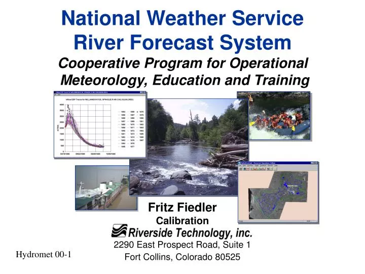
National Weather Service River Forecast System Cooperative Program for Operational Meteorology, Education and Training. Fritz Fiedler Calibration 2290 East Prospect Road, Suite 1 Fort Collins, Colorado 80525. Hydromet 00-1. Calibration. Calibration process

E N D
National Weather ServiceRiver Forecast SystemCooperative Program for Operational Meteorology, Education and Training Fritz Fiedler Calibration 2290 East Prospect Road, Suite 1 Fort Collins, Colorado 80525 Hydromet 00-1
Calibration • Calibration process • Estimation of parameter values which will minimize differences between observed and simulated streamflows • Calibration problems • Parameter interaction • Non-unique solutions • Time-consuming • Inaccuracies • Non-linearities • Lack of understanding
Calibration Continued... • Goals • Unbiased reproduction of historical conditions • Parameters that cause model components to mimic the hydrologic processes they were designed to represent • Ability to extrapolate beyond conditions encountered in historical record • To do this, must understand the watershed processes as they relate to model structure
Calibration System Parameter estimation/optimization and watershed simulation • Input • Point or areal estimates of historical precipitation, temperature, and potential evaporation • Initial hydrologic conditions • Output • Basin areal averages for point value inputs • Simulated hydrographs for historical analysis or use in ESP • Parameter values for models in operational forecast and ESP systems
Calibration System (continued) • Characteristics • Performs computations for few forecast points for many time steps • Uses operations table • Compatible with operational system and ESP • Produces graphical output for manual calibration • Includes algorithms for automatic optimization • Applications • Historical watershed simulation • Model calibration
Model Calibration • Basin-Wide Strategy • Select river system • Prepare data • MAP - Mean Areal Precipitation • MAT - Mean Areal Temperature • PE - Potential Evaporation • QME - Mean Daily Discharge • QIN - Instantaneous Discharge
Model Calibration (continued) • Calibrate least complicated headwater basins • Select calibration period • Estimate initial parameter - observed Qs • Trial and error using MCP3/ICP (Interactive) • Statistics, observed versus simulated plots • Hydrograph components • Proper approach to parameter adjustment • Automatic parameter optimization - OPT3 • Fine tuning - MCP3 • Calibrate other headwater areas • Calibrate local areas
Model Calibration (continued) • Important considerations • Model structure, simulation processes • Effects of parameter changes • Use of the forecast information
Data Preparation MAP Algorithms - Mean Areal Precipitation Techniques for converting point precipitation measurements into areal measurements and distributing them properly in time Daily and hourly data Grid point algorithm • Estimating precipitation at a point (1/D2) • Estimate: >least, <greatest • 100-150 points within basin • Normalize at each grid point, then renormalize Thiessen weights Grid point versus Thiessen Two-pass algorithm - distribute daily, then estimate missing Consistency plots MAT Algorithms - Mean Areal Temperature Max - min data Grid point algorithm (1/D) Elevation weighting factor Centroid (1/DP) Conversion to mean temperatures Consistency plots MAPE - Mean Areal Potential Evaporation Evaporation pan data MAPE vs. Mean seasonal curve QME QIN
Historical Data Analysis • General Information Needed • Station data in Calibration files • Station history info - observation times, changes, location, moves • Topog map of basin MAP Specific Information Non- Mountainous Mountains --basin boundary --isohyetal map --station weights MAT Specific Information --mean max/min temperatures Non-Mountainous Mountains --basin boundary --areal-elev curve MAPE Specific Information --Evaporation maps --mean monthly evap --station weights • PXPP • check consistency • compute normals • MAT3 • check consistency • MAPE • check consistency • generate daily time • series of MAPE • TAPLOT3 • get mean max/min for • mean zone elevation • MAP3 • (re)check consistency • generate time series • of MAP • MAT3 • generate time • series of MAT Temperature Evaporation Precipitation
E T Demand Precipitation Input Px Impervious Area E T Direct Runoff PCTIM ADIMP Pervious Area Impervious Area Upper Zone Surface Runoff EXCESS Tension Water UZTW Free Water UZFW E T UZK Interflow E T Percolation Zperc. Rexp Total Channel Inflow Distribution Function E T RIVA Streamflow 1-PFREE PFREE Lower Zone Free Water Tension Water P S LZTWLZFP LZFS RSERV Supplemental Base flow LZSK E T LZPK Total Baseflow Primary Baseflow Side Subsurface Discharge Sacramento Model Structure
Impervious and Direct Runoff Surface Runoff Interflow Discharge Supplemental Baseflow Primary Baseflow Time Hydrograph Decomposition
SAC-SMA Model Precipitation Impervious and Direct Runoff Pervious Impervious Surface Runoff Evaporation Upper Zone Interflow Supplemental Baseflow Lower Zone Primary Baseflow Sacramento Soil Moisture Components
Initial Parameter Estimates By Hydrograph Analysis (continued) LZSK - Supplemental baseflow recession (always > LZPK) Flow that typically persists anywhere from 15 days to 3 or 4 months
Initial Parameters Estimates by Hydrograph Analysis (continued)
Initial Soil Moisture Estimates by Hydrograph Analysis (continued)
Interactive Calibration Strategy • Remove large biases that may mask other problems • Adjust baseflow parameters • Adjust tension water capacities • Adjust parameters to get proper storm runoff simulation • Final adjustments to improve seasonal and flow interval bias statistics
Calibrated Models in Forecasting • Data Issues • Differences in Raingauge Networks • New/Removed Stations; Mountainous Areas • Examine Effect on MAP Seasonal Statistics • Differences in Measurement Sensors • Radar • Use of Forecast rather than Observed Precipitation • Adjust for Biases, Estimate Uncertainty • Differences in Spatial and Temporal Resolution
INTERACTIVE vs. AUTOMATIC • Model fit to data • Treats model as non-linear regression • Not labor intensive • Small number of statistical criteria • Highly sensitive to data quality • Uncertain value of future simulations • Process representation • Requires knowledge of physical model basis • Labor intensive • Multiple performance criteria • Less affected by data quality • Good potential for reliable future simulations