Download
1 / 46
460 likes | 462 Vues
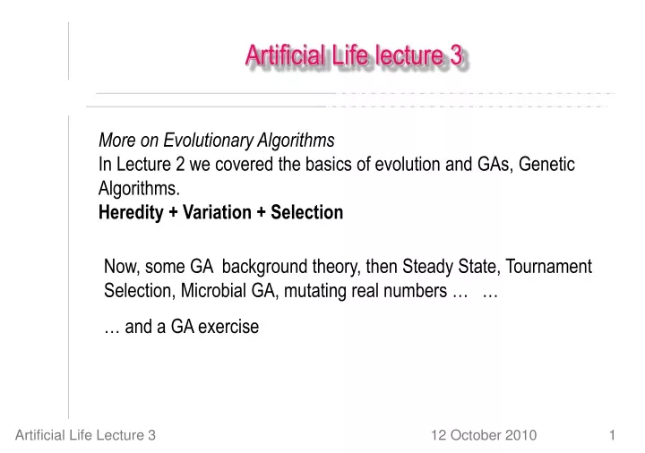
Artificial Life lecture 3. More on Evolutionary Algorithms In Lecture 2 we covered the basics of evolution and GAs, Genetic Algorithms. Heredity + Variation + Selection. Now, some GA background theory, then Steady State, Tournament Selection, Microbial GA, mutating real numbers … …

E N D
Artificial Life lecture 3 More on Evolutionary Algorithms In Lecture 2 we covered the basics of evolution and GAs, Genetic Algorithms. Heredity + Variation + Selection Now, some GA background theory, then Steady State, Tournament Selection, Microbial GA, mutating real numbers … … … and a GA exercise Artificial Life Lecture 3
Why Should GAs work ? John Holland (1975) 'Adaptation in Natural and Artificial Systems' -- and most of the textbooks -- explain this with the Schema Theorem, and ideas of building blocks. Roughly speaking, building blocks are segments of the genotype which encode for functional components of the 'phenotype', or potential solution to the problem. These building blocks can, in principle, be evaluated independently of all the rest, as varying between 'good' and 'bad'. Artificial Life Lecture 3
Cartoon Version Cartoon version of genotypes: *** long legs *****************short arms********** ***short legs***************** long arms ********** ^ Recombination (when crossover happens to land appropriately) allows different parents like these in one generation to produce a child with long legs and long arms Artificial Life Lecture 3
Schemata Schemata (plural of schema) are a formalisation of this idea of a building block. Consider binary genotypes of length 16. Let # be a 'wild-card' or 'dont-care' character. Then #####00#010##### is a schema of order 5 (5 specified alleles) and of defining length 6 (length of segment which includes specified alleles). Artificial Life Lecture 3
‘Processing Schemata’ Considering this schema #####00#010##### then 0000000001010000 is just one of many genotypes corresponding to this schema -- and actually this genotype also corresponds simultaneously to many other schemata. Implicitly, the GA 'evaluates' and 'processes' loads of schemata in parallel, every generation. Artificial Life Lecture 3
The Schema Theorem claims … ... that schemata of short defining lengths (coding for building blocks such as 'cartoon legs') will, • IF they are of above-average fitness, (..that is, evaluated whatever the other loci outside the schema are) • get exponentially increasing numbers of trials in successive generations. Ie, despite recombination and mutation being 'disruptive' (tho not too disruptive of short schemata) 'good building blocks' will multiply and take over --- and 'mix and match' with other 'good building blocks'. Artificial Life Lecture 3
Implications of the Schema Theorem ?? The Schema Theorem is formally proved subject to certain conditions. This Theorem is widely interpreted as implying that RECOMBINATION is the 'powerhouse' of GAs, -- whereas mutation is just a 'background operator‘ (whose only role is to add variety in loci where, throughout the whole population, no variety is left). Artificial Life Lecture 3
Doubts about the Schema Theorem The Schema Theorem is formally correct. But nowadays many people (including myself) believe it has been misinterpreted. The 'subject to certain conditions' bit means that this exponential increase is only guaranteed over 1 generation -- thereafter the conditions change! Artificial Life Lecture 3
Recombination versus Mutation ? So be aware that despite this common view in the textbooks, some people think that in some sense MUTATION is the powerhouse of GAs, with recombination as a background (tho often useful) genetic operator. "The Schema Theorem is true, but not very significant" Nevertheless, the common view of the importance of recombination lies behind the exclusive emphasis (often without any mutation) on recombination in GP = Genetic Programming. Now for the Microbial Genetic Algorithm Artificial Life Lecture 3
First, some more GA wrinkles You need not have a generational GA (where the whole population is swept aside every generation, and replaced by a fresh lot of offspring). You can have a STEADY STATE GA. Here just ONE member of the population is replaced at each time step, by the offspring of some others. Artificial Life Lecture 3
Steady State GA Eg with a popn of 100: • Choose a mum by some selection mechanism biased towards the fitter. • Choose a dad by same method. • Generate a child by recombination + mutation • Add the child to the population • Keep the numbers down to 100 by choosing someone else to die (eg at random, or biased towards the less fit) Roughly speaking, 100 times round this loop is equivalent to one generation of a generational GA Artificial Life Lecture 3
Tournament Selection Here is a very simple way to implement the equivalent of linear rank selection in a Steady State GA 3.5 compare fitnesses 2.7 Pick 2 at random Fittest of tournament is mum – choose dad the same way Generate offspring from mum and dad – the new offspring replaces someone chosen at random. Note: everyone else remains, including mum and dad. Repeat until happy! Artificial Life Lecture 3
The Evolutionary Mechanics All you need is a population of replicating individuals, with Heredity, Variation, and Selection. Classically in a GA, Selection was done in a Fitness-proportionate way:- 7/S 5/S 6/S 5/S … … 6/S expectation of being parent S = Sum of popn fitnesses 7 6 6 Problems:- What about negative fitnesses? The ‘Scaling problem’? 5 5 … … Artificial Life Lecture 3
Rank Selection ? Just line up all of them in Rank Order of fitness … Allocate ‘expectation of being a parent’ in proportion to their Rank. Typically linear:- the Best 2/n the Median 1/n the Worst 0/n. That’s better ― but need to Sort the population Artificial Life Lecture 3
Pick 2 at random Find the Fittest of those 2 And take that one as a Parent Tournament selection ? From the whole population It turns out that if you repeat this n times (with replacement), everyone has same expectation of parenthood as with Linear Rank Selection – and the coding is simpler! Artificial Life Lecture 3
… … … … … … The Microbial GA will use: Steady State Instead of a Generational GA, replacing all n at the same time You can just produce one new offspring at a time, replacing one. Repeat n times for the equivalent of one generation Artificial Life Lecture 3
… … AND unlike usual GAs: we will Select who dies Typically, many GAs select positively (‘greater fitness’) for who is to be a parent But it works just as well to select parents at random, then select negatively (‘less fitness’) to choose who makes way for the offspring. Artificial Life Lecture 3
Pick 2 at random as parents Generate an offspring Then select negatively which parent dies (‘less fitness’) To make way for the baby Combine these with Tournament Selection From the whole population Artificial Life Lecture 3
Without Death ― Horizontal Transmission Normally we think of Vertical Transmission of genes, from one generation to the next But Microbes can achieve the same end, without dying ! Artificial Life Lecture 3
Microbial Sex Instead of “Let’s make babies !” It is “Want to share some of my genes?” Let’s put this altogether in a very simple GA Artificial Life Lecture 3
Compare Pick W L ranked Recombine W unchanged W L Mutate Replace L mutated L ‘infected’ The Microbial GA population Artificial Life Lecture 3
Microbial Genetic Algorithm – the algorithm • Pick two genotypes at random • Compare scores -> Winner and Loser • Go along genotype, at each locus • with some prob copy from Winner to Loser (overwrite) • with some prob mutate that locus of the Loser So ONLY the Loser gets changed (gives a version of Elitism for free!) This allows what is technically a one-liner GA (bar the evaluate(), which is problem-specific) -- quite a long line ! Artificial Life Lecture 3
Microbial Genetic Algorithm – the one-liner /* tournament loop */ for (t=0;t<END;t++) /* loop along genotype of winner of tournament, selected in initial loop conditions */ for (W=(evaluate(a=POP*drand48())> evaluate(b=POP*drand48()) ? a : b), L=(W==a ? b : a), i=0; i<LEN; i++) /* throw dice to decide: cross or mutate */ if ((r=drand48())<REC+MUT) /* update genotype of loser */ gene[L][i]=(r<REC ? gene[W][i] : gene[L][i]^1); Artificial Life Lecture 3
… or slightly longer int gene[POP][LEN]; Initialise genes at random; define problem-specific evaluate(n) /* tournament loop */ for (t=0;t<END;t++) { /* pick 2 at random, find Winner and Loser */ a=POP*drand48(); do {b=POP*drand48()} while (a==b); /*make sure a and b different */ if (evaluate(a) > evaluate(b)) {W=a; L=b;} else {W=b; L=a;} To be continued … Artificial Life Lecture 3
… continued Continued … for (i=0;i<LEN;i++) { if (drand48()<REC) /* cross with probability REC */ gene[L][i]=gene[W][i]; if (drand48()<MUT) /* mutate with probability MUT */ gene[L][i]=1-gene[L][i]; /* flip bit */ } /* end tournament loop */ Possible values for REC=0.5; ? And MUT=1.0/LEN; (If Binary) ? Artificial Life Lecture 3
Compare Pick W L ranked Recombine W unchanged W L Mutate Replace L mutated L ‘infected’ The Microbial GA population Artificial Life Lecture 3
Computationally, this is really easy … … because we can keep all the genotypes in a fixed array. Only the Loser’s genotype is changed, within the array. One cycle round the loop changes one individual, n cycles is equivalent to a generation. It’s going to be so simple, we can afford to do one more trick ! Artificial Life Lecture 3
‘Trivial Geography’ If the population is not pan-mictic, but instead dispersed into (overlapping) demes, we can maintain more diversity across the whole population. GA people usually use a 2-D geography, but it looks like 1-D (a ring) is good enough (Spector & Klein) We can incorporate this still within minimal program code Artificial Life Lecture 3
Pick + Demes Compare Recombine Mutate The code void microbial_tournament(void) { int A,B,W,L,i; A=P*rnd(); // Choose A randomly B=(A+1+D*rnd())%P; // B from Deme, %P.. if (eval(A)>eval(B)) {W=A; L=B;} // ..for wrap-around else {W=B; L=A;} // W=Winner L=Loser for (i=0;i<N;i++) { // walk down N genes if (rnd()<REC) // RECombn rate gene[L][i]=gene[W][i]; // Copy from Winner if (rnd()<MUT) // MUTation rate gene[L][i]^1; // Flip a bit } } That’s all there is ! Artificial Life Lecture 3
That’s a GA with Rank Selection, Demes, Recombination, Mutation – also Elitism for free! (the current fittest never gets changed) Extensions Showing off: in 16-pt type I can do it allin 1 line of code:- for (t=0;t<T;t++) for (W=(e(A=P*r())>e(B=(A+1+D*r())%P)?A:B),L=(W==A?B:A),i=0;i<L;i++) if ((r=r())<R+M) g[L][i]=(r<R?g[W][i]:g[L][i]^1); Horizontal (microbial) Transmission allows experimentation with different rates of ‘Recombination’ (or ‘Infection’) ― need not be 50%, try anything between 0% and 100%, with different implications. Artificial Life Lecture 3
Is there a point ? Microbial GA papers on my home page http://www.cogs.susx.ac.uk/users/inmanh [cite: Harvey, I. (2009 In Press). The Microbial Genetic Algorithm.In G. Kampis et al (Eds.) Proceedings of the Tenth European Conference on Artificial Life, Springer LNCS.] It does actually work. By no means guaranteed to be better than other GAs -- but does show how really simple a GA can be, and still work ! Apart from the one line, it needs declaration of gene[POP][LEN], initialisation of a random popn, and evaluate(n) that returns fitness of nth member. Artificial Life Lecture 3
Embodied Evolution Richard Watson, at Brandeis (papers available on web) has modified this to use with real robots in 'Embodied Evolution'. Robots go around 'broadcasting' their genes, and listening out to other broadcasts. Fitter robots 'shout louder' (or more often) Weaker robots are more likely to listen in, and use the genes they 'hear' to copy over their own. Artificial Life Lecture 3
Choosing how to encode the Genotype When faced with a new problem, if you are going to tackle it with a GA then one of the first decisions is: How can I sensibly encode different phenotypes (possible solutions) as genotypes (artificial DNA, strings of symbols) ? E.g., in a Developmental System examples (eg: later lecture on L-Systems), the symbols may be appropriate for an L-system rule – the ‘artificial DNA’ is a string including [brackets] in pairs. Then it is necessary for genetic operators such as mutations to respect the encoding – cannot mutate just one side of a pair of brackets. Artificial Life Lecture 3
The purpose of the Genotype – Phenotype encoding There are many possible ways (P) to solve your problem – many ways to build a plant, a neural network, a transmission tower … You want to encode these different ways as different strings of symbols (G) so that Heredity and Variation work properly. As far as possible, small changes in G (mutations) should make small changes in P. And inheriting bits of G from different parents should ideally result in inheriting bits of each parent’s Phenotypic characteristics. Artificial Life Lecture 3
Binary versus Real-valued encoding Often we want to encode numbers on the genotype. Lecture 2 discussed encoding real numbers as bits on a genotype (either binary encoding or Gray coding) Sometimes people choose to have real numbers directly represented on the genotype -- which might be: 2.034 -30.678 0.005 102.567 ... ... -89.432 Recombination will work in the same way as with normal discretely encoded genotypes, but mutations will be handled differently. Artificial Life Lecture 3
Mutating Real numbers Various possibilities for mutating real numbers One possibility is to change any mutated locus to a randomly chosen real number within the appropriate range -- but this is very disruptive. So more usually a form of 'creep mutation' is used: eg. add a random number in range [-0.1 +0.1] or add a random number drawn from a Gaussian distribution with mean zero, and appropriate range. Artificial Life Lecture 3
Mutation Rate for real numbers In lecture 2, I suggested as a guideline that for binary encodings a good rule of thumb was: “mutn rate very approx 1 mutn per (non-junk part of) genotype” Flip-a-bit, 0↔1, big change, do it rarely on the genotype With real numbers, the rule of thumb is different: “apply a small creep rate at EVERY locus on the genotype” Small change at each locus, so do it everywhere Artificial Life Lecture 3
Evolution Strategies If the problem you are tackling has all the parameters naturally expressed as real numbers, then maybe you should investigate Evolution Strategies (see lecture 2) These work primarily with a version of 'creep mutation', and this evolutionary paradigm has developed sophisticated strategies for modifying the amounts of 'creep' in different dimensions as evolution proceeds. Artificial Life Lecture 3
Different Search Algorithms Or indeed you could look at Simulated Annealing -- a non-evolutionary technique which nevertheless has some similarities. These are all techniques for Search within a many-dimensional, real-valued Search Space. Genetic Algorithms may be more appropriate for Search within high-dimensional Discrete Search Spaces. Many design problems are such – but many are not. Artificial Life Lecture 3
Fitness Function When faced with a new problem, your first decision was: How can I sensibly encode different phenotypes (possible solutions) as genotypes (artificial DNA, strings of symbols) ? But then your second decision will have to be: How can I sensibly give a score to each member of the population, how can I evaluate its fitness ? This is a problem-dependent decision, no firm rules. Usually several different ways, some more sensible than others. This where you have to use your sense and discretion! Artificial Life Lecture 3
Genetic Algorithm Exercise Coursework for all on the Artificial Life course, to be handed in by Tue Oct 19th. Based on Lectures 2 and 3, and intended to get all of you actually implementing and running for real a very basic GA. See http://www.informatics.susx.ac.uk/users/inmanh/easy/alife10 The Card Problem (or Alternative that follows – pick 1) You have 10 cards numbered from 1 to 10. You have to choose a way of dividing them into 2 piles, so that the cards in Pile_0 *sum* to a number as close as possible to 36, and the remaining cards in Pile_1 *multiply* to a number as close as possible to 360. Artificial Life Lecture 3
Issues to consider • Genotype encoding:Each card can be in Pile_0 or Pile_1, there are 1024 possible ways of sorting them into 2 piles, and you have to find the best. Think of a sensible way of encoding any possible solution-attempt as a genotype. • Fitness:Some of these solution-attempts will be closer to the target than others. Think of a sensible way of evaluating any solution-attempt and scoring it with a fitness-measure. • The GA:Write a program, in any sensible programming language, to run a GA with your genotype encoding and Fitness function. Run it 100 times and see what results you get. Artificial Life Lecture 3
The Report • Hand in your program (the shorter the better!) and summary of your results. Plus a brief paragraph justifying the Fitness function you chose, and another brief paragraph discussing the significance of your results. • To be handed in to me by Tue Oct 19th, the Tue lecture. • OR you can do problem 2 instead (a different kind of fitness landscape)… Artificial Life Lecture 3
For Experts … … • For those who are already GA experts: • What is an optimum mutation rate? Why? • What is an optimum population size? Why? • Is it sensible to use a GA on this problem? Why? • How does search time scale up, 10/100/1000 cards? Why? • Are there punctuated equilibria in the evolutionary dynamics? Why? • Was your GA more complex than the Microbial? Why? Artificial Life Lecture 3
Alternative problem 2 You have 4 variables, that represent possible parameter settings for the design of an aircraft wing. A B C D, each of which can be any whole number between 0 and 63 (…. Think, 6 bits, 000000 to 111111 for each) Your aerodynamics model tells you that the Lift of the wing is Lift = [ A3 + 3*A*(B-C) + (D-A)4 -2*C*D ] / [3*C*D – 5*B2] (… actually, I just invented an equation rather arbitrarily … !! ) Find values of A B C D, each within their allowed range 0-63, that maximise the Lift. Artificial Life Lecture 3
Advance Reading for seminars Week 3 Check the website www.informatics.susx.ac.uk/users/inmanh/easy/alife10/index.html Artificial Life Lecture 3