Download
1 / 25
250 likes | 519 Vues
Introduction to High-Precision GPS Data Analysis: Towards a common language for the workshop. Topics to be Covered in the Workshop Wednesday Morning Introduction to GPS Data Analysis Automatic Processing using sh_gamit and sh_glred What’s New in GAMIT/GLOBK Wednesday Afternoon

E N D
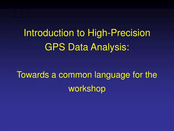
Introduction to High-Precision GPS Data Analysis: Towards a common language for the workshop
Topics to be Covered in the Workshop Wednesday Morning Introduction to GPS Data Analysis Automatic Processing using sh_gamit and sh_glred What’s New in GAMIT/GLOBK Wednesday Afternoon Reference Frames and Spatial Filtering Effective Use of GLOBK Thursday Morning Estimating Heights and Atmospheric Parameters An Approach to Error Analysis Thursday Afternoon Overview of Kinematic Processing with Track A Short Introduction to Block Modeling GAMIT/GLOBK Utilities
Your location is: 37o 23.323’ N 122o 02.162’ W Instantaneous positioning with GPS Instantaneous Positioning with Pseudoranges Receiver solution or sh_rx2apr • Point position ( svpos ) 30-100 m • Differential ( svdiff ) 3-10 m
High-precision positioning uses the phase observations• Long-session static: change in phase over time carries most of the information• Repairing cycle slips is therefore essential • The shorter the occupation, the more important is overall ambiguity resolution Each Satellite (and station) has a different signature
Accuracy of Single-baseline Observations as a Function of Session Length Horizontal Vertical Agreement in mm of single session with average of 30 24-h sessions for three different reference stations at 30, 200, and 500 km Firuzabadi & King [2009]
Horizonal (mm) Accuracy of Network Observations as a Function of Session Length Bottom labels are different reference networks (3-20 sites) with maximum extent in km Vertical (mm) Firuzabadi & King [2009]
Observables in Data Processing Fundamental observations L1 phase = f1 x range (19 cm) L2 phase = f2 x range (24 cm) C1 or P1 pseudorange used separately to get receiver clock offset (time) To estimate parameters use doubly differenced LC = 2.5 L1 - 2.0 L2 “Ionosphere-free combination” Double differencing removes clock fluctuations; LC removes almost all of ionosphere Both DD and LC amplify noise (use L1, L2 directly for baselines < 1 km) Auxiliary combinations for data editing and ambiguity resolution “Geometry-free combination” or “Extra wide-lane” (EX-WL) (86 cm) LG = L2 - f2/f1 L1 Removes all frequency-independent effects (geometric & atmosphere) but not multipath or ionosphere N2 - N1 “Widelane ambiguities” (86 cm); if phase only, includes ionosphere Melbourne-Wubbena wide-Lane (86 cm): phase/pseudorange combination that removes geometry and ionosphere; dominated by pseudorange noise
Modeling the ObservationsI. Conceptual/Quantitative • Motion of the satellites • Earth’s gravity field ( flattening 10 km; higher harmonics 100 m ) • Attraction of Moon and Sun ( 100 m ) • Solar radiation pressure ( 20 m ) • Motion of the Earth • Irregular rotation of the Earth ( 5 m ) • Luni-solar solid-Earth tides ( 30 cm ) • Loading due to the oceans, atmosphere, and surface water and ice ( 10 mm) • Propagation of the signal • Neutral atmosphere ( dry 6 m; wet 1 m ) • Ionosphere ( 10 m but cancels to few mm most of the time ) • Variations in the phase centers of the ground and satellite antennas ( 10 cm) * incompletely modeled
Modeling the ObservationsII. Software Structure • Satellite orbit • IGS tabulated ephemeris (Earth-fixed SP3 file) [ track ] • GAMIT tabulated ephemeris ( t-file ): numerical integration by arc in inertial space, fit to SP3 file, may be represented by its initial conditions (ICs) and radiation-pressure parameters; requires tabulated positions of Sun and Moon • Motion of the Earth in inertial space [model or track] • Analytical models for precession and nutation (tabulated); IERS observed values for pole position (wobble), and axial rotation (UT1) • Analytical model of solid-Earth tides; global grids of ocean and atmospheric tidal loading • Propagation of the signal [model or track ] • Zenith hydrostatic (dry) delay (ZHD) from pressure ( met-file, VMF1, or GPT ) • Zenith wet delay (ZWD) [crudely modeled and estimated in solve or track ] • ZHD and ZWD mapped to line-of-sight with mapping functions (VMF1 grid or GMT) • Variations in the phase centers of the ground and satetellite antennas (ANTEX file)
Parameter Estimation • Phase observations [ solve or track ] • Form double difference LC combination of L1 and L2 to cancel clocks & ionosphere • Apply a priori constraints • Estimate the coordinates, ZTD, and real-valued ambiguities • Form M-W WL and/or phase WL with ionospheric constraints to estimate and resolve the WL (L2-L1) integer ambiguities [ autcln, solve, track ] • Estimate and resolve the narrow-lane (NL) ambiguities • Estimate the coordinates and ZTD with WL and NL ambiguities fixed --- Estimation can be batch least squares [ solve ] or sequential (Kalman filter [ track ] • Quasi-observations from phase solution (h-file) [ globk ] • Sequential (Kalman filter) • Epoch-by-epoch test of compatibility (chi2 increment) but batch output
Limits of GPS Accuracy • Signal propagation effects • Signal scattering ( antenna phase center / multipath ) • Atmospheric delay (mainly water vapor) • Ionospheric effects • Receiver noise • Unmodeled motions of the station • Monument instability • Loading of the crust by atmosphere, oceans, and surface water • Unmodeled motions of the satellites • Reference frame
Limits of GPS Accuracy • Signal propagation effects • Signal scattering ( antenna phase center / multipath ) • Atmospheric delay (mainly water vapor) • Ionospheric effects • Receiver noise • Unmodeled motions of the station • Monument instability • Loading of the crust by atmosphere, oceans, and surface water • Unmodeled motions of the satellites • Reference frame
Reflected Signal Direct Signal Reflected Signal Mitigating Multipath Errors • Avoid Reflective Surfaces • Use a Ground Plane Antenna • Use Multipath Rejection Receiver • Observe for many hours • Remove with average from many days
Multipath and Water Vapor Effects in the Observations One-way (undifferenced) LC phase residuals projected onto the sky in 4-hr snapshots. Spatially repeatable noise is multipath; time-varying noise is water vapor. Red is satellite track. Yellow and green positive and negative residuals purely for visual effect. Red bar is scale (10 mm).
Limits of GPS Accuracy • Signal propagation effects • Signal scattering ( antenna phase center / multipath ) • Atmospheric delay (mainly water vapor) • Ionospheric effects • Receiver noise • Unmodeled motions of the station • Monument instability • Loading of the crust by atmosphere, oceans, and surface water • Unmodeled motions of the satellites • Reference frame
Monuments Anchored to Bedrock are Critical for Tectonic Studies (not so much for atmospheric studies) Good anchoring: Pin in solid rock Drill-braced (left) in fractured rock Low building with deep foundation Not-so-good anchoring: Vertical rods Buildings with shallow foundation Towers or tall building (thermal effects)
Annual Component of Vertical Loading Atmosphere (purple) 2-5 mm Snow/water (blue) 2-10 mm Nontidal ocean (red) 2-3 mm From Dong et al. J. Geophys. Res., 107, 2075, 2002
24-hr position estimates over 3 months for station in semi-arid eastern Oregon Random noise is ~1 mm horizontal, 3 mm vertical, but the vertical has ~10-level systematics lasting 10-30 days which are likely a combination of monument instability and atmospheric and hydrologic loading
Limits of GPS Accuracy • Signal propagation effects • Signal scattering ( antenna phase center / multipath ) • Atmospheric delay (mainly water vapor) • Ionospheric effects • Receiver noise • Unmodeled motions of the station • Monument instability • Loading of the crust by atmosphere, oceans, and surface water • Unmodeled motions of the satellites • Reference frame
GPS Satellite Limits to model are non-gravitational accelerations due to solar and albedo radiation, unbalanced thrusts, and outgassing; and non-spherical antenna pattern
Quality of IGS Final Orbits 1994-2008 20 mm = 1 ppb Source: http://acc.igs.org
Quality of real-time predictions from IGS Ultra-Rapid orbits 2001-2008 20 mm = 1 ppb Source: http://acc.igs.org
Limits of GPS Accuracy • Signal propagation effects • Signal scattering ( antenna phase center / multipath ) • Atmospheric delay (mainly water vapor) • Ionospheric effects • Receiver noise • Unmodeled motions of the station • Monument instability • Loading of the crust by atmosphere, oceans, and surface water • Unmodeled motions of the satellites • Reference frame
Reference Frames Global Center of Mass ~ 30 mm ITRF ~ 2 mm, < 1 mm/yr Continental < 1 mm/yr horiz., 2 mm/yr vert. Local -- may be self-defined
Effect of Orbital and Geocentric Position Error/Uncertainty High-precision GPS is essentially relative ! Baseline error/uncertainty ~ Baseline distance x geocentric SV or position error SV altitude SV errors reduced by averaging: Baseline errors are ~ 0.2 • orbital error / 20,000 km e.g. 20 mm orbital error = 0.2 ppb or 0.2 mm on 1000 km baseline Network position errors magnified for short sessions e.g. 5 mm position error ~ 1 ppb or 1 mm on 1000 km baseline 10 cm position error ~ 20 ppb or 1 mm on 50 km baseline