Download
1 / 34
820 likes | 2.5k Vues
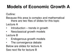
Models of Economic Growth B. Outline: 1. Endogenous growth models – Slides 1-22 (these slides offer a slightly more detailed treatment of endogenous models than Chapter 8) 2. The convergence debate – Slides 23 – 34 (this is additional to material covered in the book).

E N D
Models of Economic Growth B Outline: 1. Endogenous growth models – Slides 1-22 (these slides offer a slightly more detailed treatment of endogenous models than Chapter 8) 2. The convergence debate – Slides 23 – 34 (this is additional to material covered in the book)
Endogenous growth models - topics • Recap on growth of technology (A) in Solow model (…..does allow long run growth) • Endogenous growth models • Non-diminishing returns to ‘capital’ • Role of human capital • Creative destruction models • Competition and growth • Scale effects on growth
Exogenous technology growth • Solow (and Swan) models show that technological change drives growth • But growth of technology is not determined within the model (it is exogenous) • Note that it does not show that capital investment is unimportant ( A y and MPk, hence k) • In words …. better technology raises output, but also creates new capital investment opportunities • Endogenous growth models try to make endogenous the driving force(s) of growth • Can be technology or other factors like learning by workers
The AK model • The ‘AK model’ is sometimes termed an ‘endogenous growth model’ • The model has Y = AK where K can be thought of as some composite ‘capital and labour’ input • Clearly this has constant marginal product of capital (MPk = dY/dK=A), hence long run growth is possible • Thus, the ‘AK model’ is a simple way of illustrating endogenous growth concept • However, it is very simple! ‘A’ is poorly defined, yet critical to growth rate • Also composite ‘K’ is unappealing
Endogenous technology growth • Suppose that technology depends on past investment (i.e. the process of investment generates new ideas, knowledge and learning). If a+b = 1 then marginal product of capital is constant (dY/dK = L1-a ).
Assuming A=g(K) is Ken Arrow’s (1962) learning-by-doing paper • Intuition is that learning about technology prevents marginal product declining
Situation on growth diagram Distance between lines represents growth in capital per worker
Increasing returns to scale • “Problem” with Y = K1L1-a is that it exhibits increasing returns to scale (doubling K and L, more than doubles Y) • IRS large firms dominate, no perfect competition (no P=MC, no first welfare theorem, …..) • …. solution, assume feedback from investment to A is external to firms (note this is positive externality, or spillover, from microeconomics)
Knowledge externalities • Romer (1986) paper formally proves such a model has a competitive equilibrium • However, the importance of externalities in knowledge (R&D, technology) long recognised • Endogenous growth theory combines IRS, knowledge externalities and competitive behaviour in (dynamic optimising) models
More formal endogenous growth models • Romer (1990), Jones (1995) and others use a model of profit-seeking firms investing in R&D • A firm’s R&D raises its profits, but also has a positive externality on other firms’ R&D productivity (can have competitive behaviour at firm-level, but IRS overall) • Assume Y=Ka(ALY)1-a • Labour used either to produce output (LY) or technology (LA) • As before, A is technology (also called ‘ideas’ or ‘knowledge’) • Note total labour supply is L = LY + LA
Romer model Note ‘knife edge’ property of f=1. If f>1, growth rate will accelerate over time; if f<1, growth rate falls.
Jones model (semi-endogenous) • No scale effects, no ‘knife edge’ property, but requires (exogenous) labour force growth hence “semi-endogenous” (see Jones (1999) for discussion)
Human capital – the Lucas model • Lucas defines human capital as the skill embodied in workers • Constant number of workers in economy is N • Each one has a human capital level of h • Human capital can be used either to produce output (proportion u) • Or to accumulate new human capital (proportion 1-u) • Human capital grows at a constant rate dh/dt = h(1-u)
Lucas model in detail • The production of output (Y) is given by Y = AKα (uhN)1-α ha g where 0 < a < 1 and g 0 • Lucas assumed that technology (A) was constant • Note the presence of the extra term hag - this is defined as the ‘average human capital level’ • This allows for external effect of human capital that can also influence other firms, e.g. higher average skills allow workers to communicate better • Main driver of growth - As h grows the effect is to scale up the input of workers N, so raising output Y and raising marginal product of capital K
Creative destruction and firm-level activity • many endogenous growth models assume profit-seeking firms invest in R&D (ideas, knowledge) • Incentives: expected monopoly profits on new product or process. This depends on probability of inventing and, if successful, expected length of monopoly (strength of intellectual property rights e.g. patents) • Cost: expected labour cost (note that ‘cost’ depends on productivity, which depends on extent of spillovers) • models are ‘monopolistic competitive’ i.e. free entry into R&D zero profits (fixed cost of R&D=monopoly profits). ‘Creative destruction’ since new inventions destroy markets of (some) existing products. • without ‘knowledge spillovers’ such firms run into diminishing returns • such models have three potential market failures, which make policy implications unclear
Market failures in R&D growth models • Appropriability effect (monopoly profits of a new innovation < consumer surplus) too little R&D • Creative-destruction, or business stealing, effect (new innovation destroys profits of existing firms), which private innovator ignores too much R&D • Knowledge spillover effect (each firm’s R&D helps reduce costs of others innovations; positive externality) too little R&D The overall outcome depends on parameters and functional form of model
What do we learn from such models? • Growth of technology via ‘knowledge spillovers’ vital for economic growth • Competitive profit-seeking firms can generate investment & growth, but can be market failures (‘social planner’ wants to invest more since spillovers not part of private optimisation) • Spillovers, clusters, networks, business-university links all potentially vital • But models too generalised to offer specific policy guidance
Competition and growth • Endogenous growth models imply greater competition, lower profits, lower incentive to do R&D and lower growth (R&D line shifts down) • But this conflicts with economists’ basic belief that competition is ‘good’! • Theoretical solution • Build models that have optimal ‘competition’ • Aghion-Howitt model describes three sector model (“escape from competition” idea) • Intuitive idea is that ‘monopolies’ don’t innovate
Do ‘scale effects’ exist • Romer model implies countries that have more ‘labour’ in knowledge-sector (e.g. R&D) should grow faster • Jones argues this not the case (since researchers in US 5x (1950-90) but growth still 2% p.a. • Hence, Jones claims his semi-endogenous model better fits the ‘facts’, BUT • measurement issues (formal R&D labs increasingly used) • ‘scale effects’ occur via knowledge externalities (these may be regional-, industry-, or network-specific) • Kremer (1993) suggests higher population (scale) does increase growth rates over last 1000+ years • anyhow…. both models show f (the ‘knowledge spillover’ parameter) is important
Questions for discussion • What is the ‘knife edge’ property of endogenous growth models? • Is more competition good for economic growth? • Do scale effects mean that China’s growth rate will always be high?
References Arrow, K. (1962). "The Economic Consequences of Learning by Doing." Review of Economic Studies XXIX(80): 155-173. Jones, C. (1995). "R&D Based Models of Economic Growth." Journal of Political Economy 103(4): 759-784. Jones, C. (1999) "Growth: With or Without Scale Effects?" American Economic Review Papers and Proceedings, 89, 139-144. Kremer, M. (1993). "Population Growth and Technological Change: One Million B.C. to 1990." Quarterly Journal of Economics 108: 681-716. Lucas, R. E. (1988). "On the Mechanics of Economic Development." Journal of Monetary Economics 22: 3-42. Mankiw, N., D. Romer, et al. (1992). "A Contribution to the Empirics of Economic Growth." Quarterly Journal of Economics 107(2): 407-437. Romer, P. (1986). "Increasing Returns and Long Run Growth." Journal of Political Economy 94(2): 1002-1037. Romer, P. (1990). "Endogenous Technological Change." Journal of Political Economy 98(5): S71-S102.
Convergence debate • Following slides discuss the above issue, which is not included in detail in book • However, it may be a topic to include in a course on macroeconomics of growth, see: • Milanovic, B. (2002). "Worlds Apart: Inter-National and World Inequality 1950-2000". World Bank, http://www.worldbank.org/research/inequality/world%20income%20distribution/world%20apart.pdf. • Pritchett, L. (1997). "Divergence, Big Time." Journal of Economic Perspectives 11(3): 3-17. • Stiglitz, J.-E. (2000). "Capital Market Liberalization, Economic Growth, and Instability." World Development 28(6): 1075-86.
Do poorer countries grow faster? (the ‘convergence’ debate) Two common ways to assess convergence • Beta (b) convergence • Sigma (s) convergence b-convergence (use regression analysis) growthi = constant + b (initial GDP p.w.)i (i stands for a country. Test on sample of 60+) If b<0, poorer countries, on average, grow faster s-convergence measure dispersion (variance) of GDP per worker across countries in a given year. If dispersion falls over time can say countries ‘converging’.
b-convergence, 110 countries, 1965-2000 Source: PWT 6.1 Estimated b for above = 0.000. No beta convergence
Problems and other evidence • There are more than 110 countries (UN 191). The poorest countries often don’t have data. Hence above result could be mis-leading. • L Pritchett (1997) “Divergence, Big Time”. • 1870-1990, rich countries got much richer • 9/1 ratio in 1870; 45/1 ratio in 1990 • Some view the 1960s-80s as good decades for poorer countries – normally divergence • “Conditional convergence”. • If regression analysis controls for other factors (e.g. investment), poorer countries do grow faster. • Not very surprising …. what are other factors?
sigma (s) convergence • Variance (110 countries GDP per worker) increases over time divergence since 60s • But, if you weight countries according to population, evidence shows convergence (this appears entirely due to China, Milanovic, 2002, see next slide) (note: if you do not weight you give China and, say, Togo the same ‘importance’ or ‘weight’) • Finally, researchers now working on ‘true’ world inequality data (i.e. combine within country, and across country, inequality). Initial results show ‘world’ inequality increasing since late 1980s
Gini measure of inter-country inequality Source: Data direct from Branko Milanovic, see Milanovic (2002). The higher the Gini-coefficient, the more ‘unequal’ is GDP per capita across the world (see endnotes)
Twin peaks ? Some evidence that world income distribution is moving to ‘twin-peaks’ distribution…… but not very strong 1995 real GDP per worker 1965 real GDP per worker
What are mechanisms driving ‘convergence’? • Important to understand basic data, but real issue is mechanisms • Consider some ‘theory’ initially • open economy growth models • models of technological catch-up • Note: this ‘convergence’ is not ‘Solow-Swan convergence to steady state’ • can consider country convergence in S-S model but must assume technology common to all countries
Weighted world inter-country inequality (role of China and India)
Summary (I) Sigma (s) convergence • Using unweighted measures, cross-country evidence suggests ‘divergence’ • Weighted measures convergence over last 30 years due to performance of China • However, most recent ‘world inequality’ measures based on within and across country data, divergence
Summary (II) Beta (b) convergence • No unconditional convergence • There is conditional convergence (poorer countries grow faster if you control for other factors) • Expect this (basic closed economy Solow and endogenous growth models predict this)
Endnotes Inequality/Convergence • Gini coefficient, world income inequality. • The Gini coefficient varies from 0 (perfect equality) to 1 (perfect inequality). • The discussion related to this overlooks many important and controversial issues. See Milanovic (2002) for a discussion, or google it. • Milanovic, B. (2002). "Worlds Apart: Inter-National and World Inequality 1950-2000". World Bank, http://www.worldbank.org/research/inequality/world%20income%20distribution/world%20apart.pdf.