Download

1 / 43
590 likes | 1.34k Vues
Aggregate Planning. 13. PowerPoint presentation to accompany Heizer and Render Operations Management, 10e Principles of Operations Management, 8e PowerPoint slides by Jeff Heyl. Frito-Lay.

E N D
Aggregate Planning 13 PowerPoint presentation to accompany Heizer and Render Operations Management, 10e Principles of Operations Management, 8e PowerPoint slides by Jeff Heyl © 2011 Pearson Education, Inc. publishing as Prentice Hall
Frito-Lay • More than three dozen brands, 15 brands sell more than $100 million annually, 7 sell over $1 billion • Planning processes covers 3 to 18 months • Unique processes and specially designed equipment • High fixed costs require high volumes and high utilization © 2011 Pearson Education, Inc. publishing as Prentice Hall
Frito-Lay • Demand profile based on historical sales, forecasts, innovations, promotion, local demand data • Match total demand to capacity, expansion plans, and costs • Quarterly aggregate plan goes to 38 plants in 18 regions • Each plant develops 4-week plan for product lines and production runs © 2011 Pearson Education, Inc. publishing as Prentice Hall
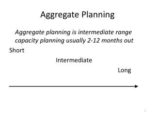
Aggregate Planning The objective of aggregate planning is to meet forecasted demand while minimizing cost over the planning period © 2011 Pearson Education, Inc. publishing as Prentice Hall
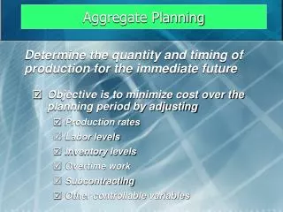
The Planning Process Determine the quantity and timing of production for the intermediate future • Objective is to minimize cost over the planning period by adjusting • Production rates • Labor levels • Inventory levels • Overtime work • Subcontracting rates • Other controllable variables © 2011 Pearson Education, Inc. publishing as Prentice Hall
Aggregate Planning Required for aggregate planning • A logical overall unit for measuring sales and output • A forecast of demand for an intermediate planning period in these aggregate terms • A method for determining costs • A model that combines forecasts and costs so that scheduling decisions can be made for the planning period © 2011 Pearson Education, Inc. publishing as Prentice Hall
Quarter 1 Jan Feb Mar 150,000 120,000 110,000 Quarter 2 Apr May Jun 100,000 130,000 150,000 Quarter 3 Jul Aug Sep 180,000 150,000 140,000 Aggregate Planning © 2011 Pearson Education, Inc. publishing as Prentice Hall
Aggregate Planning Figure 13.2 © 2011 Pearson Education, Inc. publishing as Prentice Hall
Aggregate Planning • Combines appropriate resources into general terms • Part of a larger production planning system • Disaggregation breaks the plan down into greater detail • Disaggregation results in a master production schedule © 2011 Pearson Education, Inc. publishing as Prentice Hall
Aggregate Planning Strategies Use inventories to absorb changes in demand Accommodate changes by varying workforce size Use part-timers, overtime, or idle time to absorb changes Use subcontractors and maintain a stable workforce Change prices or other factors to influence demand © 2011 Pearson Education, Inc. publishing as Prentice Hall
Capacity Options • Changing inventory levels • Increase inventory in low demand periods to meet high demand in the future • Increases costs associated with storage, insurance, handling, obsolescence, and capital investment • Shortages may mean lost sales due to long lead times and poor customer service © 2011 Pearson Education, Inc. publishing as Prentice Hall
Capacity Options • Varying workforce size by hiring or layoffs • Match production rate to demand • Training and separation costs for hiring and laying off workers • New workers may have lower productivity • Laying off workers may lower morale and productivity © 2011 Pearson Education, Inc. publishing as Prentice Hall
Capacity Options • Varying production rate through overtime or idle time • Allows constant workforce • May be difficult to meet large increases in demand • Overtime can be costly and may drive down productivity • Absorbing idle time may be difficult © 2011 Pearson Education, Inc. publishing as Prentice Hall
Capacity Options • Subcontracting • Temporary measure during periods of peak demand • May be costly • Assuring quality and timely delivery may be difficult • Exposes your customers to a possible competitor © 2011 Pearson Education, Inc. publishing as Prentice Hall
Capacity Options • Using part-time workers • Useful for filling unskilled or low skilled positions, especially in services © 2011 Pearson Education, Inc. publishing as Prentice Hall
Demand Options • Influencing demand • Use advertising or promotion to increase demand in low periods • Attempt to shift demand to slow periods • May not be sufficient to balance demand and capacity © 2011 Pearson Education, Inc. publishing as Prentice Hall
Demand Options • Back ordering during high- demand periods • Requires customers to wait for an order without loss of goodwill or the order • Most effective when there are few if any substitutes for the product or service • Often results in lost sales © 2011 Pearson Education, Inc. publishing as Prentice Hall
Demand Options • Counterseasonal product and service mixing • Develop a product mix of counterseasonal items • May lead to products or services outside the company’s areas of expertise © 2011 Pearson Education, Inc. publishing as Prentice Hall
Aggregate Planning Options Table 13.1 © 2011 Pearson Education, Inc. publishing as Prentice Hall
Aggregate Planning Options Table 13.1 © 2011 Pearson Education, Inc. publishing as Prentice Hall
Aggregate Planning Options Table 13.1 © 2011 Pearson Education, Inc. publishing as Prentice Hall
Aggregate Planning Options Table 13.1 © 2011 Pearson Education, Inc. publishing as Prentice Hall
Methods for Aggregate Planning • A mixed strategy may be the best way to achieve minimum costs • There are many possible mixed strategies • Finding the optimal plan is not always possible © 2011 Pearson Education, Inc. publishing as Prentice Hall
Mixing Options to Develop a Plan • Chase strategy • Match output rates to demand forecast for each period • Vary workforce levels or vary production rate • Favored by many service organizations © 2011 Pearson Education, Inc. publishing as Prentice Hall
Mixing Options to Develop a Plan • Level strategy • Daily production is uniform • Use inventory or idle time as buffer • Stable production leads to better quality and productivity • Some combination of capacity options, a mixed strategy, might be the best solution © 2011 Pearson Education, Inc. publishing as Prentice Hall
Graphical Methods • Popular techniques • Easy to understand and use • Trial-and-error approaches that do not guarantee an optimal solution • Require only limited computations © 2011 Pearson Education, Inc. publishing as Prentice Hall
Graphical Methods Determine the demand for each period Determine the capacity for regular time, overtime, and subcontracting each period Find labor costs, hiring and layoff costs, and inventory holding costs Consider company policy on workers and stock levels Develop alternative plans and examine their total costs © 2011 Pearson Education, Inc. publishing as Prentice Hall
Total expected demand Number of production days Average requirement = 6,200 124 = = 50 units per day Roofing Supplier Example 1 Table 13.2 © 2011 Pearson Education, Inc. publishing as Prentice Hall
Forecast demand 70 – 60 – 50 – 40 – 30 – 0 – Level production using average monthly forecast demand Production rate per working day Jan Feb Mar Apr May June = Month 22 18 21 21 22 20 = Number of working days Roofing Supplier Example 1 Figure 13.3 © 2011 Pearson Education, Inc. publishing as Prentice Hall
Roofing Supplier Example 2 Plan 1 – constant workforce Table 13.3 © 2011 Pearson Education, Inc. publishing as Prentice Hall
Roofing Supplier Example 2 Total units of inventory carried over from one month to the next = 1,850 units Workforce required to produce 50 units per day = 10 workers Plan 1 – constant workforce Table 13.3 © 2011 Pearson Education, Inc. publishing as Prentice Hall
Roofing Supplier Example 2 Total units of inventory carried over from one month to the next = 1,850 units Workforce required to produce 50 units per day = 10 workers Plan 1 – constant workforce Table 13.3 © 2011 Pearson Education, Inc. publishing as Prentice Hall
7,000 – 6,000 – 5,000 – 4,000 – 3,000 – 2,000 – 1,000 – – Reduction of inventory 6,200 units Cumulative level production using average monthly forecast requirements Cumulative demand units Cumulative forecast requirements Excess inventory Jan Feb Mar Apr May June Roofing Supplier Example 2 Figure 13.4 © 2011 Pearson Education, Inc. publishing as Prentice Hall
Roofing Supplier Example 3 Table 13.2 Plan 2 – subcontracting Minimum requirement = 38 units per day © 2011 Pearson Education, Inc. publishing as Prentice Hall
Forecast demand 70 – 60 – 50 – 40 – 30 – 0 – Level production using lowest monthly forecast demand Production rate per working day Jan Feb Mar Apr May June = Month 22 18 21 21 22 20 = Number of working days Roofing Supplier Example 3 © 2011 Pearson Education, Inc. publishing as Prentice Hall
Roofing Supplier Example 3 Table 13.3 © 2011 Pearson Education, Inc. publishing as Prentice Hall
Roofing Supplier Example 3 In-house production = 38 units per day x 124 days = 4,712 units Subcontract units = 6,200 - 4,712 = 1,488 units Table 13.3 © 2011 Pearson Education, Inc. publishing as Prentice Hall
Roofing Supplier Example 3 In-house production = 38 units per day x 124 days = 4,712 units Subcontract units = 6,200 - 4,712 = 1,488 units Table 13.3 © 2011 Pearson Education, Inc. publishing as Prentice Hall
Roofing Supplier Example 4 Table 13.2 Plan 3 – hiring and layoffs Production = Expected Demand © 2011 Pearson Education, Inc. publishing as Prentice Hall
Forecast demand and monthly production 70 – 60 – 50 – 40 – 30 – 0 – Production rate per working day Jan Feb Mar Apr May June = Month 22 18 21 21 22 20 = Number of working days Roofing Supplier Example 4 © 2011 Pearson Education, Inc. publishing as Prentice Hall
Roofing Supplier Example 4 Table 13.3 © 2011 Pearson Education, Inc. publishing as Prentice Hall
Roofing Supplier Example 4 Table 13.3 Table 13.4 © 2011 Pearson Education, Inc. publishing as Prentice Hall
Comparison of Three Plans Plan 2 is the lowest cost option Table 13.5 © 2011 Pearson Education, Inc. publishing as Prentice Hall