PID Control for Embedded Systems

PID Control for Embedded Systems Richard Ortman and John Bottenberg

The Problem • Add/change input to a system • Did it react how you expected? • Could go to fast or slow • External environmental factors can play a role (i.e. gravity)

Feedback Control • Say you have a system controlled by an actuator • Hook up a sensor that reads the effect of the actuator(NOT the output to the actuator) • You now have a feedback loop and can use it to control your system! Sensor Actuator http://en.wikipedia.org/wiki/File:Simple_Feedback_02.png

Example: Robotic Arm Potentiometer Reads 0 to 5 V Robot Motor/Gearbox Takes -12 to 12 V PWM later http://www.chiefdelphi.com/media/photos/27132 Tell this arm to go to a specified angle

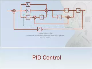
Introduction to PID • Stands for Proportional, Integral, and Derivative control • Form of feedback control http://en.wikipedia.org/wiki/File:PID_en_updated_feedback.svg

Simple Feedback Control (Bad) double Control (double setpoint, double current) { double output; if (current < setpoint) output = MAX_OUTPUT; else output = 0; return output; } • Why won't this work in most situations?

Simple Feedback Control Fails • Moving parts have inertia • Moving parts have external forces acting upon them (gravity, friction, etc)

Proportional Control • Get the error - the distance between the setpoint (desired value) and the actual value • Multiply it by Kp, the proportional gain • That's your output! double Proportional(double setpoint, double current, double Kp) { double error = setpoint - current; double P = Kp * error; return P; }

Set-point (5V) Actuator + potentiometer Actual (2V) Error (3V)

Proportional Tuning • If Kp is too large, the sensor reading will rapidly approach the setpoint, overshoot, then oscillate around it • If Kp is too small, the sensor reading will approach the setpoint slowly and never reach it

What can go wrong? • When error nears zero, the output of a P controller also nears zero • Forces such as gravity and friction can counteract a proportional controller and make it so the setpoint is never reached (steady-state error) • Increased proportional gain (Kp) only causes jerky movements around the setpoint

Proportional-Integral Control • Accumulate the error as time passes and multiply by the constant Ki. That is your I term. Output the sum of your P and I terms. double PI(double setpoint, double current, double Kp, double Ki) { double error = setpoint - current; double P = Kp * error; static double accumError = 0; accumError += error; double I = Ki * accumError; return P + I; }

PI controller • The P term will take care of the large movements • The I term will take care of any steady-state error not accounted for by the P term

Limits of PI control • PI control is good for most embedded applications • Does not take into account how fast the sensor reading is approaching the setpoint • Wouldn't it be nice to take into account a prediction of future error?

Proportional-Derivative Control • Find the difference between the current error and the error from the previous timestep and multiply by the constant Kd. That is your D term. Output the sum of your P and D terms. double PD(double setpoint, double current, double Kp, double Kd) { double error = setpoint - current; double P = Kp * error; static double lastError = 0; double errorDiff = error - lastError; lastError = error; double D = Kd * errorDiff; return P + D; }

PD Controller • D may very well stand for "Dampening" • Counteracts the P and I terms - if system is heading toward setpoint, D term is negative! • This makes sense: The error is decreasing, so d(error)/dt is negative

PID Control • Combine P, I and D terms! double PID(double setpoint, double current, double Kp, double Ki, double Kd) { double error = setpoint - current; double P = Kp * error; static double accumError = 0; accumError += error; double I = Ki * accumError; static double lastError = 0; double errorDiff= error - lastError; lastError = error; double D = Kd * errorDiff; return P + I + D; }

Saturation - Common Mistake • PID controller can output any value, but actuator has a minimum and maximum input value double saturate(double input, double min, double max) { if (input < min) return min; if (input > max) return max; return input; } // Saturate the output of your PID function double pid = PID(setpoint, current, Kp, Ki, Kd); double output = saturate(pid, min, max); // Send this output to your actuator! Actuator = output;

Timesteps - Common Mistake

Timesteps - Common Mistake • Calling a PID control function at different or erratic frequencies results in different behavior • Regulate this by specifying dt! double PID(double setpoint, double current, double Kp, double Ki, double Kd, double dt) { double error = setpoint - current; double P = Kp * error; static double accumError = 0; accumError += error * dt; double I = Ki * accumError; static double lastError = 0; double errorDiff = (error - lastError) / dt; lastError = error; double D = Kd * errorDiff; return P + I + D; }

PID Tuning • Start with Kp = 0, Ki = 0, Kd= 0 • Tune P term - System should be at full power unless near the setpoint • Tune Ki until steady-state error is removed • Tune Kd to dampen overshoot and improve responsiveness to outside influences • PI controller is good for most embedded applications, but D term adds stability

PID Applications • Robotic arm movement (position control) • Temperature control • Speed control (ENGR 151 TableSat Project) Taken from the ENGR 151 CTools site

More information • Take EECS 461! Learn about PID transfer functions. • Great tutorial: Search "umichpid control" http://ctms.engin.umich.edu/CTMS/index.php?example=Introduction&section=ControlPID

Conclusion • PID uses knowledge about the present, past, and future state of the system, collected by a sensor, to control an actuator • In PID control, the constants Kp, Ki, and Kd must be tuned for maximum performance

Questions?

PID Control for Embedded Systems