Molecular Evolution

Molecular Evolution

Outline • Evolutionary Tree Reconstruction • “Out of Africa” hypothesis • Did we evolve from Neanderthals? • Distance Based Phylogeny • Neighbor Joining Algorithm • Additive Phylogeny • Least Squares Distance Phylogeny • UPGMA • Character Based Phylogeny • Small Parsimony Problem • Fitch and Sankoff Algorithms • Large Parsimony Problem • Maximum Likelihood Method • Evolution of Wings • HIV Evolution • Evolution of Human Repeats

Early Evolutionary Studies • Anatomical features were the dominant criteria used to derive evolutionary relationships between species since Darwin till early 1960s • The evolutionary relationships derived from these relatively subjective observations were often inconclusive. Some of them were later proved incorrect 47 million year old primate fossil found 5/17/09

Evolution and DNA Sequence Analysis: the Giant Panda Riddle • For roughly 100 years scientists were unable to figure out which family the giant panda belongs to • Giant pandas look like bears but have features that are unusual for bears and typical for raccoons, e.g., they do not hibernate • In 1985, Steven O’Brien and colleagues solved the giant panda classification problem using DNA sequences and algorithms

Evolutionary Tree of Bears and Raccoons

Out of Africa Hypothesis • Around the time the giant panda riddle was solved, a DNA-based reconstruction of the human evolutionary tree led to the Out of Africa Hypothesis thatclaims our most ancient ancestor lived in Africa roughly 200,000 years ago

Human Evolutionary Tree (cont’d) http://www.mun.ca/biology/scarr/Out_of_Africa2.htm

The Origin of Humans: ”Out of Africa” vs Multiregional Hypothesis Out of Africa: • Humans evolved in Africa ~150,000 years ago • Humans migrated out of Africa, replacing other humanoids around the globe • There is no direct descendence from Neanderthals Multiregional: • Humans migrated out of Africa mixing with other humanoids on the way • There is a genetic continuity from Neanderthals to humans • Humans evolved in the last two million years as a single species. Independent appearance of modern traits in different areas

mtDNA analysis supports “Out of Africa” Hypothesis • African origin of humans inferred from: • African population was the most diverse (sub-populations had more time to diverge) • The evolutionary tree separated one group of Africans from a group containing all five populations. • Tree was rooted on branch between groups of greatest difference.

Evolutionary Tree of Humans (mtDNA) The evolutionary tree separates one group of Africans from a group containing all five populations. Vigilant, Stoneking, Harpending, Hawkes, and Wilson (1991)

Evolutionary Tree of Humans: (microsatellites) • Neighbor joining tree for 14 human populations genotyped with 30 microsatellite loci.

Human Migration Out of Africa 1. Yorubans 2. Western Pygmies 3. Eastern Pygmies 4. Hadza 5. !Kung 1 2 3 4 5 http://www.becominghuman.org

Two Neanderthal Discoveries Feldhofer, Germany Mezmaiskaya, Caucasus Distance: 25,000km

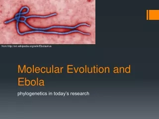
Two Neanderthal Discoveries • Is there a connection between Neanderthals and today’s Europeans? • If humans did not evolve from Neanderthals, whom did we evolve from?

Multiregional Hypothesis? • May predict some genetic continuity from the Neanderthals through to the Cro-Magnons up to today’s Europeans • Can explain the occurrence of varying regional characteristics

Sequencing Neanderthal’s mtDNA • mtDNA from the bone of Neanderthal is used because it is up to 1,000x more abundant than nuclear DNA • DNA decay overtime and only a small amount of ancient DNA can be recovered (upper limit: 100,000 years) • PCR of mtDNA (fragments are too short, human DNA may be mixed in)

Neanderthals vs Humans: Surprisingly large divergence • AMH vs Neanderthal: • 22 substitutions and 6 indels in 357 bp region • AMH vs AMH • only 8 substitutions

Evolutionary Trees How are these trees built from DNA sequences?

Evolutionary Trees How are these trees built from DNA sequences? In an evolutionary (or phylogenetic) tree, • leaves represent existing species (or taxa) • internal vertices represent ancestors (and speciation events) • root represents the oldest evolutionary ancestor • edges are sometimes called lineages

Rooted and Unrooted Trees • In an unrooted tree, the position of the root (“oldest ancestor”) is unknown. Otherwise, they are like rooted trees. We are especially interested in degree-3 (unrooted) trees because they correspond to binary phyolegenies.

Distances in Trees • Edges may have weights reflecting: • Number of mutations in the evolutionary process from one species to another • Time estimate for evolution from one species into another • In a tree T, we often compute dij(T) - the length of the path between leaves i and j dij(T) iscalled the treedistance between i and j

j i Distance in Trees: an Example d1,4 = 12 + 13 + 14 + 17 + 12 = 68

Distance Matrix • Given n species, we can compute an n x n distance matrixDij • Dij may be defined as the edit distance between a gene in species i and species j, where the gene of interest is sequenced for all n species. Dij – editdistance between i and j (min number of edit operations to transform one sequence into the other) An alignment displays how to edit one sequence into the other using operations insertion, deletion, and substitutions. The largest score implies the smallest editing cost. So, the edit distance is the complement of the optimal alignment score. ACTGGA T AGT GACT

Edit Distance vs. Tree Distance • Given n species, we can compute the n x n distance matrixDij • Dij may be defined as the edit distance between a gene in species i and species j, where the gene of interest is sequenced for all n species. Dij – editdistance between i and j • Note the difference with dij(T) – tree distance between i and j

Fitting Distance Matrix • Given n species, we can compute the n x n distance matrixDij • Evolution of these genes is described by a tree that we don’t know. • We need an algorithm to construct a tree that best fits the distance matrix Dij

Fitting Distance Matrix • Fitting means Dij = dij(T) Lengths of path in an (unknown) tree T Edit distance between species (known)

Tree reconstruction for any 3x3 matrix is straightforward We have 3 leaves i, j, k and a center vertex c Reconstructing a 3 Leaved Tree Observe: dic + djc = Dij dic + dkc = Dik djc + dkc = Djk

dic + djc = Dij + dic + dkc = Dik 2dic + djc + dkc = Dij + Dik 2dic + Djk = Dij + Dik dic = (Dij + Dik – Djk)/2 Similarly, djc = (Dij + Djk – Dik)/2 dkc = (Dki + Dkj – Dij)/2 Reconstructing a 3 Leaved Tree(cont’d)

Trees with > 3 Leaves • A degree-3 tree with n leaves has 2n-3 edges • This means fitting a given tree to a distance matrix D requires solving a system of “n choose 2” equations with 2n-3 variables • This is not always possible to solve for n > 3

Additive Distance Matrices Matrix D is ADDITIVE if there exists a tree T with dij(T) = Dij NON-ADDITIVE otherwise

Distance Based Phylogenetic Reconstruction • Goal: Reconstruct an evolutionary tree from a distance matrix • Input: n x n distance matrix Dij • Output: weighted tree T with n leaves fitting D • If D is additive, this problem has a solution and there is a simple algorithm to solve it

Find neighboring leavesi and j with parent k Remove the rows and columns of i and j Add a new row and column corresponding to k, where the distance from k to any other leaf m can be computed as: Using Neighboring Leaves to Construct the Tree Dkm = (Dim + Djm – Dij)/2 Compress i and j into k, and iterate algorithm for rest of tree

Finding Neighboring Leaves • To find neighboring leaves we could simply select a pair of closest leaves.

Finding Neighboring Leaves • To find neighboring leaves we could simply select a pair of closest leaves. WRONG

Finding Neighboring Leaves • Closest leaves aren’t necessarily neighbors • i and j are neighbors, but (dij= 13) > (djk = 12) • Finding a pair of neighboring leaves is • a nontrivial problem!

Neighbor Joining Algorithm • In 1987, Naruya Saitou and Masatoshi Nei developed a neighbor joining algorithm (NJ) for phylogenetic tree reconstruction • Finds a pair of leaves that are close to each other but far from the other leaves: implicitly finds a pair of neighboring leaves • Advantage: works well for additive and other non-additive matrices, it does not have the flawed molecular clock assumption • More details in the old slides

Degenerate Triples • A degenerate triple is a set of three distinct elements/taxa 1≤i,j,k≤n where Dij + Djk = Dik • Element j in a degenerate triple i,j,k lies on the evolutionary path from i to k (or is attached to this path by an edge of length 0).

Looking for Degenerate Triples • If distance matrix Dhas a degenerate triple i,j,k then j can be “removed” from D thus reducing the size of the problem. • If distance matrix Ddoes not have a degenerate triple i,j,k, one can “create” a degenerative triple in D by shortening all hanging edges (in the tree).

Shortening Hanging Edges to Produce Degenerate Triples • Shorten all “hanging” edges (edges that connect leaves) until a degenerate triple is found

Finding Degenerate Triples • If there is no degenerate triple, all hanging edges are reduced by the same amount δ, so that all pair-wise distances in the matrix are reduced by 2δ. • Eventually this process collapses one of the leaves (when δ = length of shortest hanging edge), forming a degenerate triple i,j,k and reducing the size of the distance matrix D. • The attachment point for j can be recovered in the reverse transformations by saving Dijfor each collapsed leaf.

Reconstructing Trees for Additive Distance Matrices

Additive Phylogeny Algorithm • AdditivePhylogeny(D) • ifD is a 2 x 2 matrix • T = tree of a single edge of length D1,2 • return T • ifD is non-degenerate • δ = trimming parameter of matrix D • for all 1 ≤ i ≠ j ≤ n • Dij = Dij - 2δ • else • δ = 0

AdditivePhylogeny (cont’d) • Find a triple i, j, k in D such that Dij + Djk = Dik • x = Dij • Remove jth row and jth column from D • T = AdditivePhylogeny(D) • Add a new vertex v to T at distance x from i to k • Add j back to T by creating an edge (v,j) of length 0 • for every leaf l in T • if distance from l to j in the tree ≠ Dl,j • output “matrix is not additive” • return • Extend all “hanging” edges by length δ • returnT

The Four Point Condition • AdditivePhylogeny provides a way to check if distance matrix D is additive • An even more efficient additivity check is the “four-point condition” • Let 1 ≤ i,j,k,l ≤ n be four distinct leaves in some (unknown) tree. This quartet induces an (unknown) 4-leaf tree where the neighboring pairs are e.g. i,j and k,l

The Four Point Condition (cont’d) Compute: 1. Dij + Dkl, 2. Dik + Djl, 3. Dil + Djk 2 3 1 2 and3represent the same number:the length of all edges + the middle edge (it is counted twice) 1represents a smaller number:the length of all edges – the middle edge

The Four Point Condition: Theorem • The four point condition for the quartet i,j,k,l is satisfied if two of these sums are the same, with the third sum smaller than these first two • Theorem (Buneman): An n x n matrix D is additive if and only if the four point condition holds for every quartet 1 ≤ i,j,k,l ≤ n • Proof in old slides

2 1 5 A B 5 3 5 4 5 Tree reconstruction based on Buneman’s Theorem Consider leaves 1,2,3,4. If then their quartet tree is: Now we insert leaf 5 into the tree, and consider quartet 1,2,3,5. If then we insert leaf 5 between ancestor A and leaf 3. But If then leaf 5 could be inserted either between A and B or between B and 2 or between B and 4. So, we need to further consider a quartet 1,2,4,5 and decide the precise edge to insert 5.

Least Squares Distance Phylogeny Problem • If the distance matrix D is NOT additive, then we look for a tree T that approximates D the best: Squared Error : ∑i,j (dij(T) – Dij)2 • Squared Error is a measure of the quality of the fit between distance matrix and the tree: we want to minimize it. • Least Squares Distance Phylogeny Problem: Finding the best approximation tree T for a non-additive matrix D (which isNP-hard).

UPGMA: Unweighted Pair Group Method with Arithmetic Mean • UPGMA is a hierarchical clustering algorithm that: • computes the distance between clusters using average pairwise distance (avg link) • assigns a height to every vertex in the tree, effectively assuming the presence of a molecular clock and dating every vertex

Clustering in UPGMA Given two disjoint clusters Ci, Cj of sequences, 1 dij = ––––––––– {p Ci, q Cj}dpq |Ci|  |Cj| Note that if Ck = Ci  Cj, then distance to another cluster Cl is: dil |Ci| + djl |Cj| dkl = –––––––––––––– |Ci| + |Cj|

Molecular Evolution