MINIMAL DEFECTS

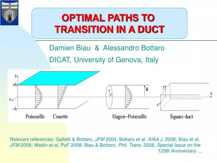
1. OPTIMAL PATHS TO TRANSITION IN A DUCT MINIMAL DEFECTS Damien Biau & Alessandro Bottaro DICAT,University of Genova,Italy Relevant references: Galletti & Bottaro, JFM 2004; Bottaro et al. AIAA J. 2006; Biau et al. JFM 2008; Wedin et al. PoF 2008; Biau & Bottaro, Phil. Trans. 2008, Special Issue on the 125th Anniversary …

2. HYDRODYNAMIC STABILITY THEORY • The flow in a duct is asymptotically stable to small perturbations • Is transient growth the solution? Butler & Farrell (1993) Trefethen, Trefethen Reddy & Driscoll (1993) Schmid & Henningson (2001) Transient growth is related to unstructured operator’s perturbations, i.e. to the pseudospectrum of the linear stability operator: [L(U, w; a, b, Re) + D] v = 0

3. The case studied dP/dx = const. characteristic length = h [channel height] characteristic speed = ut [ut2= -(h/4r) dp/dx] Ret = 150 (MARGINAL VALUE)

4. Governing equations: Linearized disturbance equations: Linearized disturbance equations:

5. OPTIMAL PERTURBATIONS: Traditional functional optimization with adjoints The adjoint problem reads:

6. G = 873,1 at t+ = 1.31 G = 869.03 at t+ = 2.09 uopt = 0 at t+ = 0 uopt≠ 0 at t+ = 0 t+ t+

7. Nonlinear evolution of the optimal disturbances ( + random noise) (streamwise periodic duct of length 4p) fully developed turbulence F = skin friction factor (F = 0.0415 from DNS at Ret = 150 (Reb = 2084)) At t = 0: a = 0 E0 = 10-1!! a = 1 E0 = 7.8 x 10-3 a = 2 E0 = 4.4 x 10-3

8. Streamwise/time averaged turbulent flow Excellent agreement with Gavrilakis, JFM 1992.

9. The a = 1 mode The threshold value is E0 = 7.8 x 10-3. In fact the optimal perturbation for a = 1 is not so important. What matters is the distorted field which emerges at t ~ 0.8. Such a field is subject to a strong amplification.

10. Partial conclusions 1 • Global optimal disturbances are interesting concepts, with probably • little connection to transition • The key to transition is to set up a distorted base flow with certain • features • The distorted base flow can be set up efficiently by sub-optimal • disturbances in the form of streamwise travelling waves. In fact, • any initial condition in the form of a travelling wave of sufficiently • large amplitude is capable to do it! • Is there any scope for studying optimal perturbations?

11. What happens past t ~ 0.8? Streamwise velocity showing a non-staggered array of L vortices (similar to H-type transition)

12. What happens past t ~ 0.8? The secondary flow does not oscillate around the 8-vortex state, but around a 4-vortex state, with active walls which alternate ... … eventually relaminarisation ensues (and the lifetime of the turbulence depends non-monotonically on the streamwise dimension of the computational box)

13. THE PHASE SPACE PICTURE EU = mean flow energy Reb = Reynolds number based on bulk velocity lower branch solution upper branch solution (qualitative)

14. Partial conclusions 2 • A saddle point appears in phase space to structure the turbulence; • after leaving the unstable manifold of the saddle, the trajectory loops • in phase space a few times, with the flow spending most of the time • in the vicinity of the saddle, until the flow eventually relaminarizes. • The lifetime depends on the box size.

15. HYDRODYNAMIC STABILITY THEORY • Distorted base flow: minimal defects Bottaro, Corbett & Luchini (2003) Biau & Bottaro (2004) Ben-Dov & Cohen (2007) The growth of instabilities on top of a distorted base flow (related to dynamical uncertainties and/or poorly modeled terms) is related to structured operator’s perturbations, i.e. to the structured pseudospectrum of the linear stability operator. [L(U, w; a, b, Re) + D] v = 0 Unstructured perturbations [L(U + DU, w; a, b, Re)] v = 0 Structured perturbations

16. Input-output framework Instead of optimising the input (the vortex), we optimise the output (the streak)!

17. SENSITIVITY ANALYSIS

18. SENSITIVITY ANALYSIS

19. MINIMAL DEFECT constraint constraint

22. We do not look directly at the spectrum of temporal eigenvalues of the direct and adjoint equations, instead we iterate the PDE’s for long time, until the leading eigenvalue emerges. Advantage: if we decided to iterate for a fixed (short) time, we could find the optimal defect for transient growth …

23. Minimal defects for e = 1, Ret = 150 (e = 1 corresponds to 0.16 of the laminar flow energy)

24. Minimum defect for a = 1: Unstable eigenmode: modulus of the streamwise streamwise vel. perturbation velocity defect (the white line corresponds to u = Ub)

25. Partial conclusions 3 • Minimal defects represent the optimisation of the output (rather than • the input, as customarily done in optimal perturbation analysis) • They can lead to transition as efficiently as suboptimal perturbations • Both minimal defects and suboptimals are more efficient for initial a‘s • larger than zero (i.e. when the disturbances have small longitudinal • dimensions) • We have not closed the cycle yet ... we need to include the feedback !

26. Self sustained process

27. A NEW OPTIMISATION APPROACH: i.e. maximising the feedback

28. The initial process of transition: • Algebraic growth of a O(e) travelling wave • Generation of weak streamwise vortices O(e2) • by quadratic interactions • Production of a strong streak O(e2Re) by lift-up • Wavy instability of the streak to close the loop • U0(y,z) U(y,z,t) u(x,y,z,t) • 0 V(y,z,t) v(x,y,z,t) • 0 W(y,z,t) w(x,y,z,t) • P0(x) P(y,z,t) p(x,y,z,t) + +

29. Inserting into the Navier-Stokes equations we obtain equations for STREAMWISE-AVERAGED FLOW plusFLUCTUATIONS

30. Goal: maximise the feedback of the wave onto the rolls, i.e. maximise Reynolds stress terms or, more simply, the energy GAIN of the wave over a fixed time interval: G = e(T)/e(0) with Tool: the usual Lagrangian optimisation, with adjoints

31. ADJOINT EQUATIONS: with SENSITIVITY FUNCTIONS

32. Ansatz for the fluctuations: acceptable as long as in the first stage of the process the large scale coherent wave is but mildly affected by the behaviour of features occurring at smaller space-time scales

33. Optimisation result for Ret = 150, a = 1, T = 1, e0 = 3x10-3 Energy of the defect Energy of the wave

34. Parametric study Defect Wave

35. Two comments:a small  defect is not created (classical optimal perturbations are of little use)a large  cut off length  “minimal channel”

36. Comparison between the minimal defect (left) and the optimal streak at t = 0.6 (centre) DNS at t = 0.6

37. Evolution of the skin friction in time turbulent mean value laminar value “edge state”

39. chaos edge laminar fixed point THE EDGE MEDIATES LAMINAR-TURBULENT TRANSITION, it is the stable manifold of the hyperbolic fixed point

40. The edge state solution

41. Simplified phase diagram

42. Global optimal perturbations saddle node state “edge states” (Wedin et al. 2007)

43. Partial conclusions 4 • A model has been developed which closes the loop and combines transient growth, exponential amplification, defects, the “exact coherent states” and the SSP • In the very initial stages of transition we need growth of a wave and • feedback onto the mean flow, to create a vortex. The lift-up then generates the streaks, which break down and re-generate the wave. • The initial conditions in the form of elongated streaks (the optimal disturbance) is inefficient at yielding transition because it fails at • modifying the mean flow • Our new simplified model yields a flow which sits initially on a trajectory directed towards the saddle point on the edge surface; direct simulations confirm the suitability of the proposed model • The basic flow structure of the edge state is two vortex pairs, overlapping one another, with the stronger pair sitting on a wall • LINEAR equations can go a long way !!!