Download
1 / 16
160 likes | 280 Vues
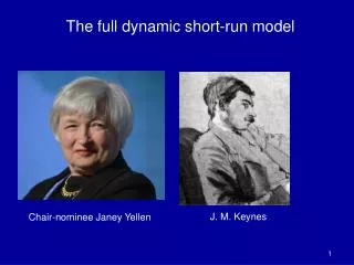
The full dynamic short-run model. The Dynamic Model. A nice new addition to Mankiw. Combines - IS - LM (changed to reflect central bank targeting) - Phillips curve Closed economy Short-run of business cycles Keynesian rather than classical. Monetary policy rule. Taylor rule:

E N D
The Dynamic Model A nice new addition to Mankiw. Combines - IS - LM (changed to reflect central bank targeting) - Phillips curve Closed economy Short-run of business cycles Keynesian rather than classical
Monetary policy rule Taylor rule: i t = πt + θπ(πt - π*) +θY (Yt - Y* ) Rationale: a rule that incorporates both real and inflation targets But, also one that has good stability properties Derived from minimizing loss function such as L = θπ(πt - π*) 2 +θY (lnYt - lnY* ) 2 [This version has loss function the same as the Taylor run. It seems more likely that the optimal Y* would be above potential output.]
Fedfunds* = pi +2 + .5*(pi – 2) - .25*(u – nairu) pi = 4 quarter PCE core inflation Why is rate below target today?
Algebra of Dynamic AS-AD analysis Key equations: 1. Demand for goods and services: Yt = Y* - α (rt –r*) + μG + εt 2. Cost of capital: rt = it – πe t + risk premium 3. Phillips curve: πt = πe t + φ(Yt - Y* ) + vt 4. Inflation expectations: πe t = π t-1 5. Monetary policy: i t = πt + θπ(πt - π*) +θY (Yt - Y* ) Notes: • Equation (1) is just our IS-LM solution • Phillips curve substitutes output by Okun’s Law • Mankiw uses slightly different version of (4) • Mankiw doesn’t consider risk premium, so ignore for now • We have added “G” to show the impact of fiscal policy
Solve for AS and AD AD: Y t = -[α θπ /(1+ α θ Y )] πt + μ /(1+ α θ Y )]G +… AS: πt = πt-1 + φ(Yt - Y* ) + vt NOTE: AD is like IS-LM equilibrium except is substitutes the Fed response for a fixed money supply AS is Phillips curve with substituting for expected inflation Note that we have moved up one derivative from intro AD-AD because of Phillips curve.
The graphics of dynamic AS-AD π AS πt* AD Yt* Y = real output (GDP)
AS Inflationary shock π AS AD Y = real output (GDP) Y*
Example by simulation model This will be available on course web page. You might download and do some experiments to see how it works. New kind of economics: computerized modeling. [The screen shots are ones that were used in class. The model posted on the course web site is slightly changed from that version.]
Other examples • Supply shocks (e-sup = 1) • Financial crisis (shock r = 1) • Inflation targeting without output targets: much deeper recessions with demand shocks (ECB) • Unstable monetary policy where insufficient response to shocks (Great Inflation discussion) • Liquidity trap
Summary This now finishes our treatment of closed-economy business cycles. Key elements are - IS elements in I, C, fiscal policy, and trade - Financial markets and monetary policy - Inflation dynamics Can we abolish the business cycle?